
Main results
Week 3: From Naive Bayes to Neural Networks
Machine learning is the study of computer algorithms that can improve automatically through experience and by the use of data
The field originated in an environment where the available data, statistical methods, and computing power rapidly and simultaneously evolved
Due to the “black box” nature of the algorithm’s operations, it is often seen as a form of artificial intelligence
Source: qlik
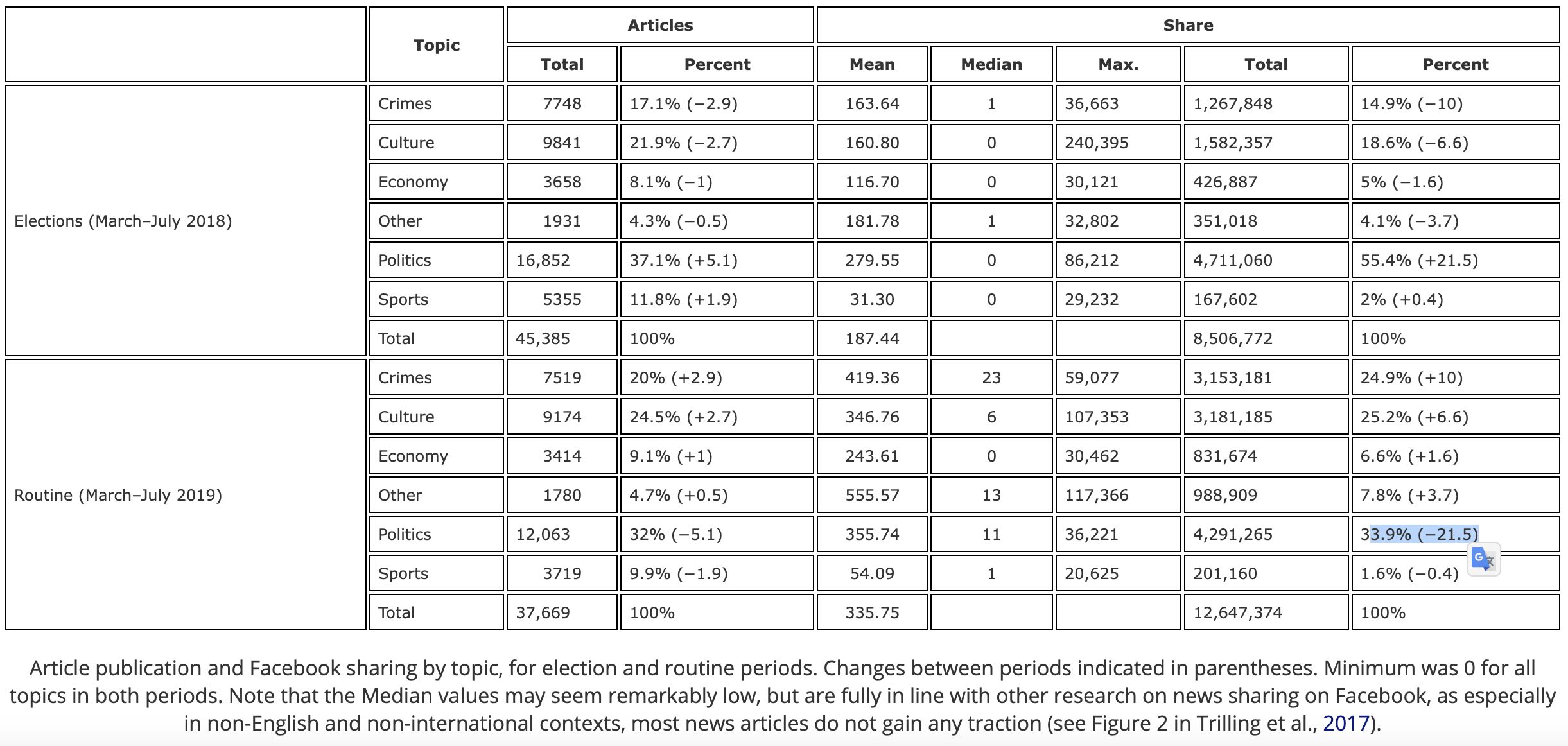
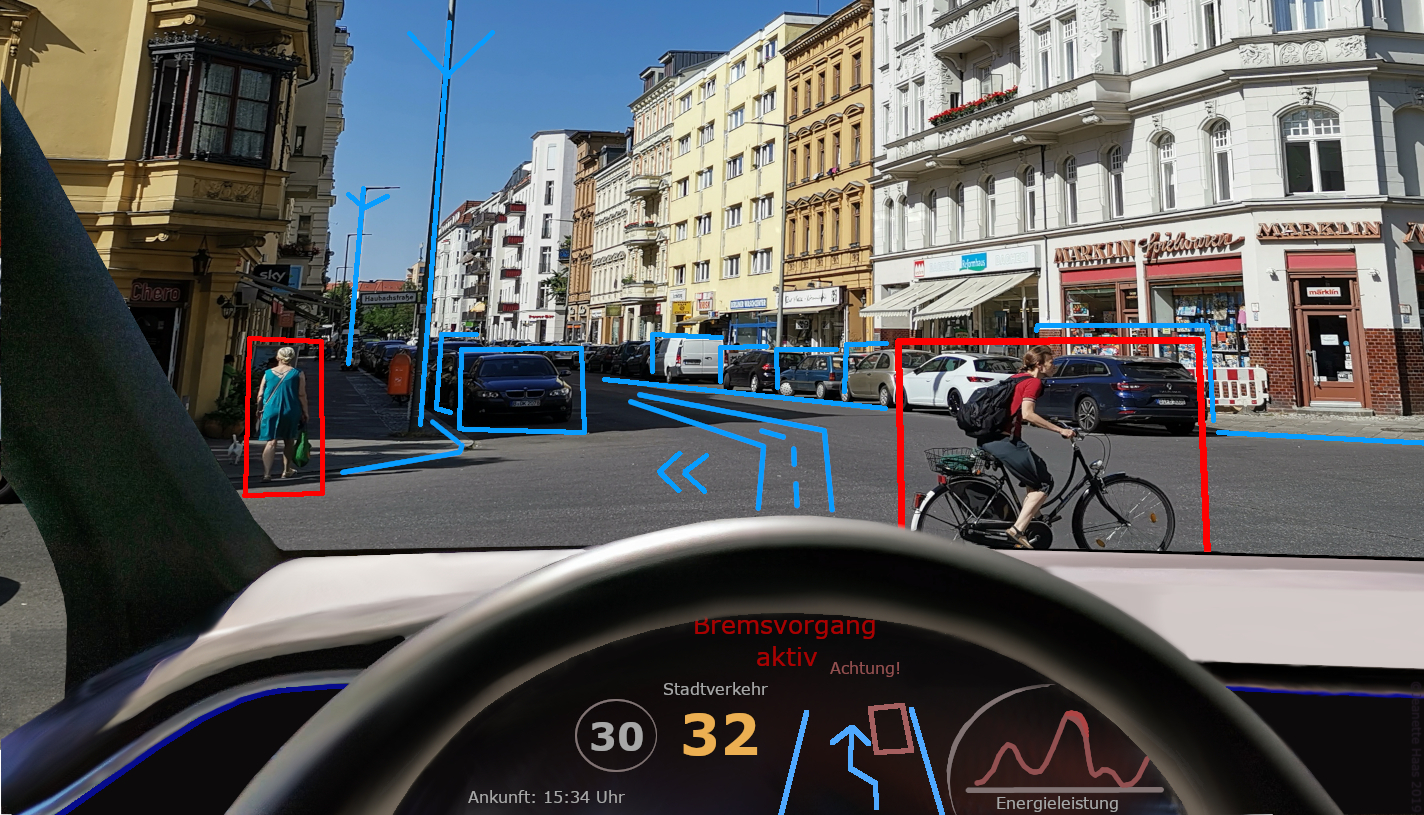 Applying machine learning in practical context:
The general goal, however, is always the same: Model the relationship between…
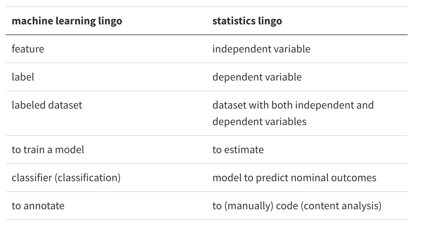
Machine learning, many people joke, is nothing other than a fancy name for statistics.
There is some truth to this: if you say “logistic regression”, this will sound familiar to both statisticians and machine learning practitioners.
Still, there are some differences between traditional statistical approaches and the machine learning approach, even if some of the same mathematical tools are used.

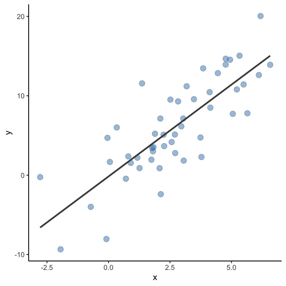
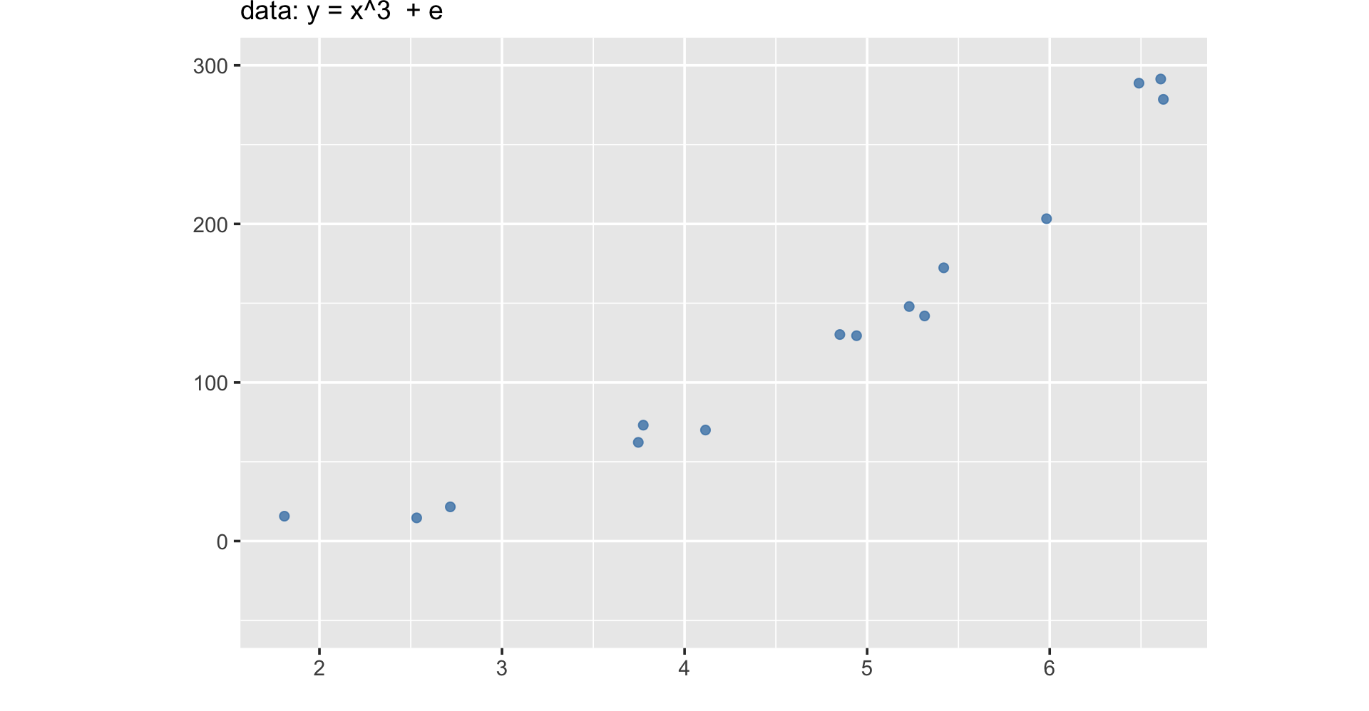
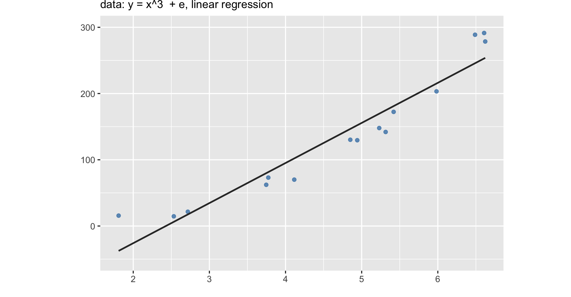
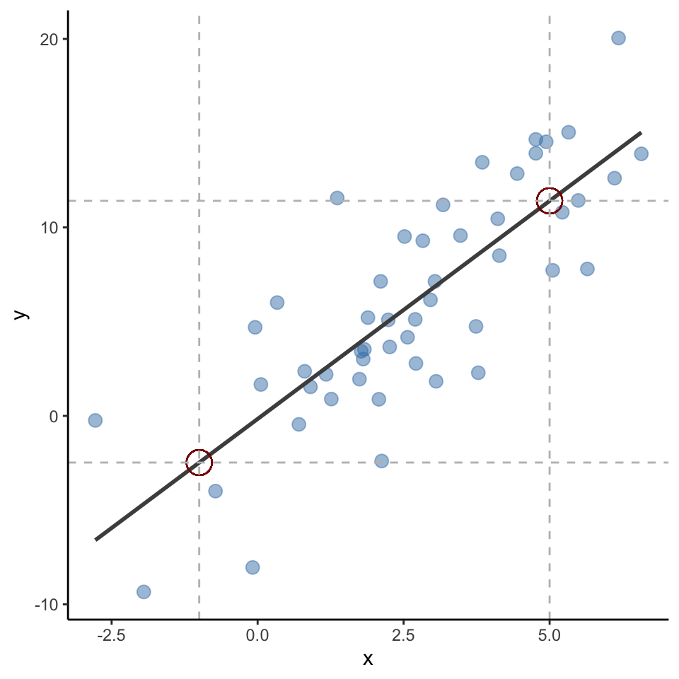
Statistical modeling is about understanding the relationship between one (or several predictors) and an outcom variable
Learn \(f\) so you can predict \(y\) from \(x\):
y based on x:x increases by one unit,y increases by 2.31 units.
Machine learning is less about understanding the relationship, but about maximizing prediction.
A statistical model such as the one estimated can be used to predict most likely y values based on new x data.
For example, despite not being in the data, x = -1 should be y = -2.47; x = 5 should be y = 11.41 based on the fitted line!
In other words, machine learnings doesn’t focus on explanation, but emphasizes prediction.
Remember how we validated dictionary approaches?
In supervised text classification, the procedure is similar
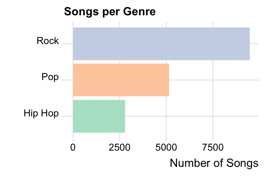
This data is scraped from the “Vagalume” website, so it depends on their storing and sharing millions of song lyrics (not really representative or complete)
Contains artist name, song name, lyrics, and genre of the artist (not the song)
The following genres are in this subsample of the data set:
library(tidytext)
lyrics_data |>
  filter(Artist == "Radiohead" & Song == "Paranoid Android") |>
  unnest_tokens(lines, text, token = "sentences") |>
  select(lines) |>
  print(n = 20)
# A tibble: 39 × 1
lines
<chr>
1 please could you stop the noise, i'm trying to get some rest.
2 from all the unborn chicken voices in my head.
3 what's this...?
4 (i may be paranoid, but not an android).
5 what's this...?
6 (i may be paranoid, but not an android).
7 when i am king, you will be first against the wall.
8 with your opinion which is of no consequence at all.
9 what's this...?
10 (i may be paranoid, but no android).
11 what's this...?
12 (i may be paranoid, but no android).
13 ambition makes you look pretty ugly.
14 kicking and squealing gucci little piggy.
15 you don't remember.
16 you don't remember.
17 why don't you remember my name?.
18 off with his head, man.
19 off with his head, man.
20 why don't you remember my name?.
# ℹ 19 more rows
There are different way to think about creating a test vs. training data set
Simplest form: split-half (or any other percentage distribution)
But there are also other, more complex procedures that fall under the term “cross-validation”
What approach is meaningful depends on the question and goal!


The collection tidymodels contains a variety of packages that facilitates and streamlines machine learning in R
The basic procedure is the following:

Goes back to the Bayes’ Theorem published in 1763!
Computes the prior probability ( P ) for every category ( c = outcome variable ) based on the training data set
Computes the probability of every feature ( x ) to be a characteristic of the class ( c ); i.e., the relative frequency of the feature in category
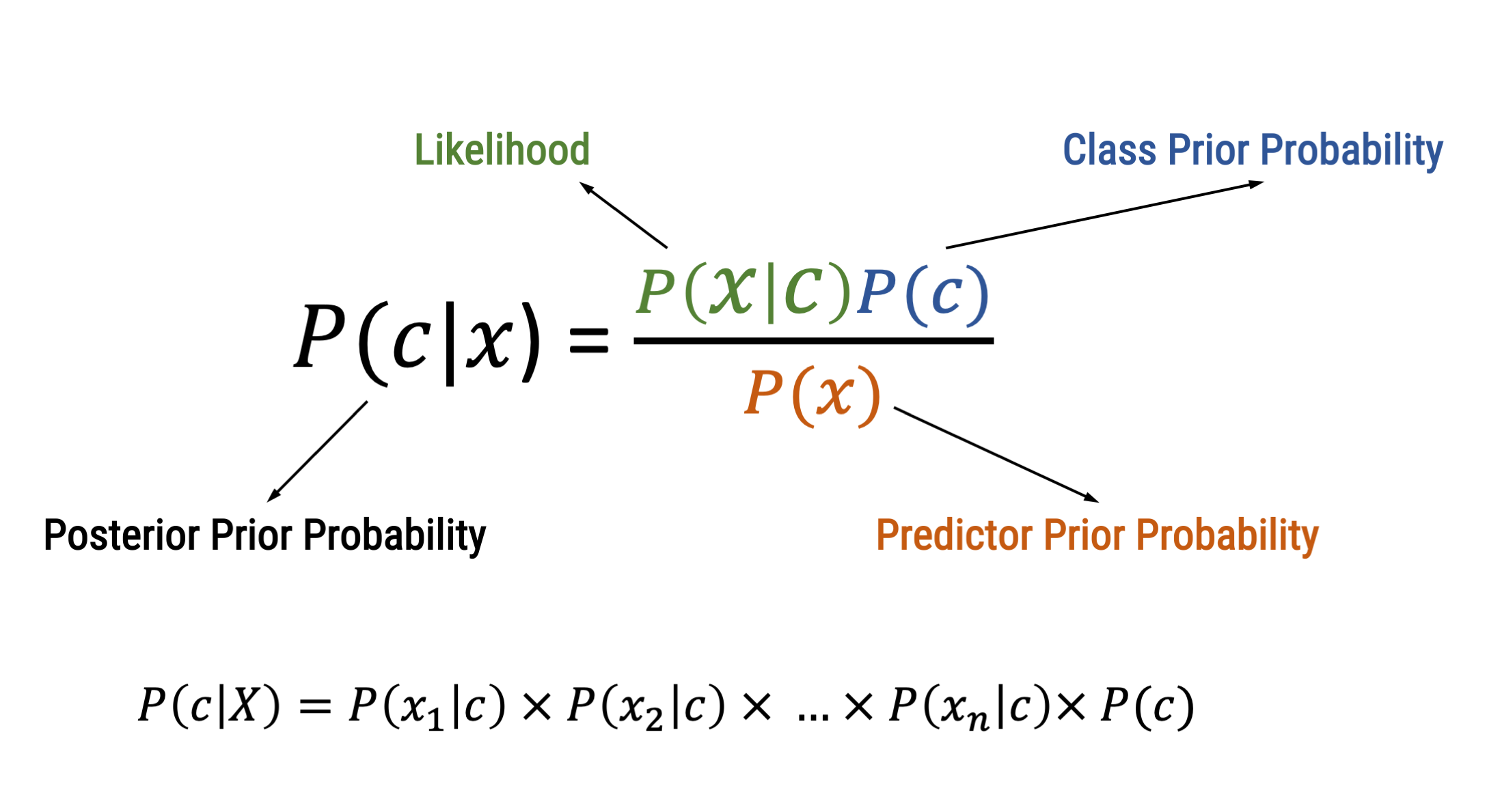
For every probability of a category in light of certain features ( P(c|X) ), all feature probabilities ( x ) are multiplied
The algorithm hence chooses the class that has highest weighted sum of inputs
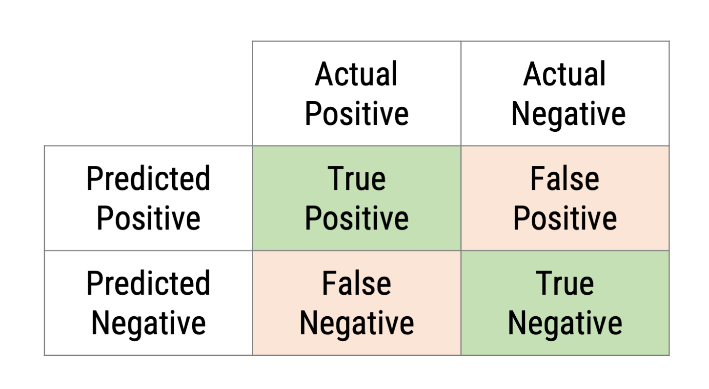
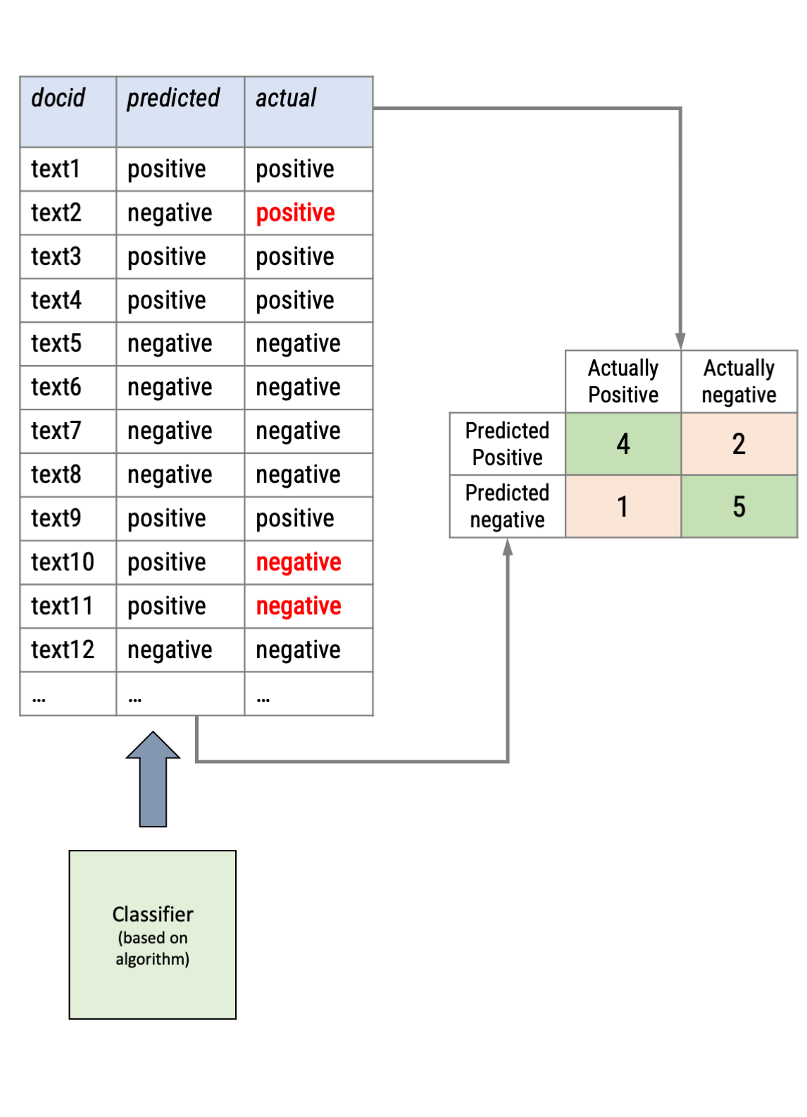
Using the function conf_mat on the actual and predicted genre columns, we can now inspect the confusion matrix
We already see that there are many “false-positives” (1890!), but less false negatives.
As mentioned earlier, a linear regression can be described with the following formula:
\(Y_i = b_0 + b_1 x_i + \epsilon_i\)
When we classify text, the dependent variable (the outcome class: \(Y_i\)) is not metric, but has only two values (1 = “is class”, 0 = “is not class”).
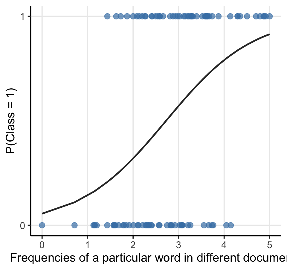
We thus need to estimate the probability of \(Y = 1\) by using the so-called sigmoid function:
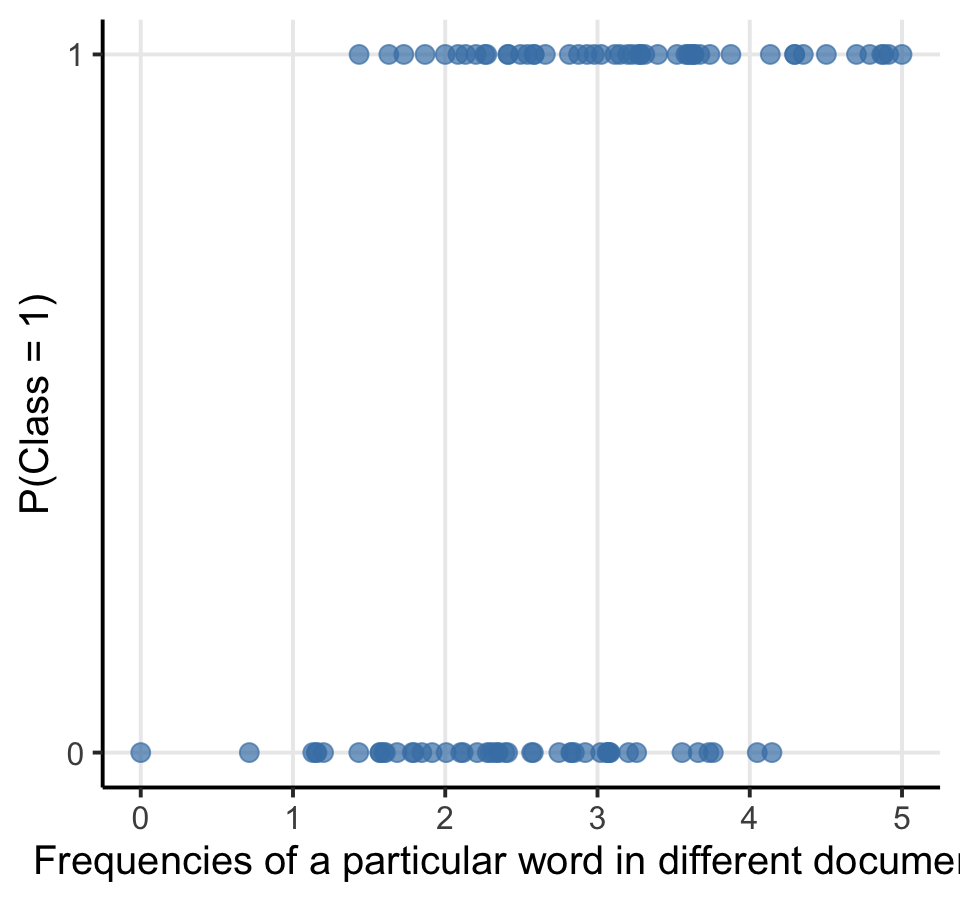
In both classic statistics as well as machine learning, this is know as logistic regression
In machine learning, we see it as an algorithm that accomplishes binary classification tasks by predicting the probability of an outcome, event, or observation
To train a classifier during text classification tasks, we simply fit a logistic regression model with all text features (e.g., the frequencies of words per document) as input (predictors) and provide the outcome class as output (dependent variable)
In contrast to statistical models that use logistic regression, the machine learning model contains thus only much more variables!
m_logistic |>
  extract_fit_parsnip() |>
  vip::vi() |>
  group_by(Sign) |>
  mutate(Sign = recode(Sign,
                       POS = "negative",
                       NEG = "positive")) |>
  top_n(20, wt = abs(Importance)) |>
  ungroup() |>
  mutate(
    Importance = abs(Importance),
    Variable = str_remove(Variable, "tf_text_"),
    Variable = fct_reorder(Variable, Importance)
  ) |>
  ggplot(aes(x = Importance,
             y = Variable,
             fill = Sign)) +
  geom_col(show.legend = FALSE) +
  facet_wrap(~Sign, scales = "free_y") +
  labs(y = NULL)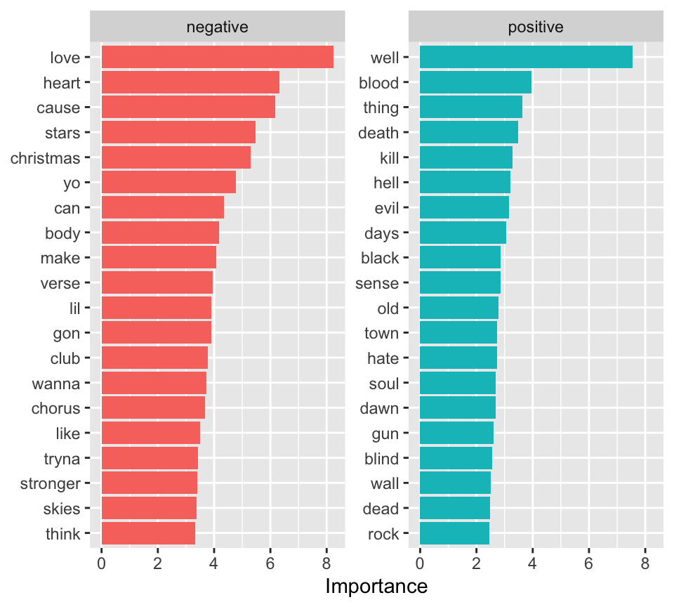
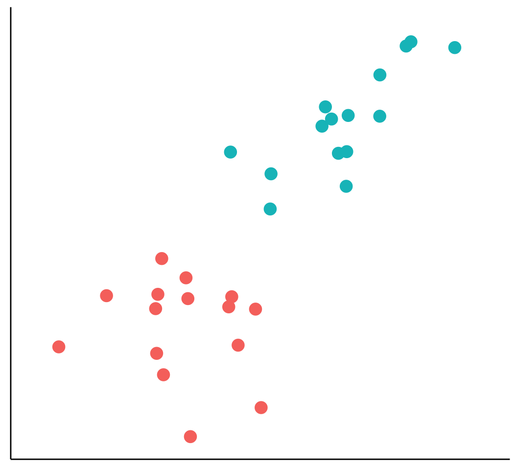
The following figure depicts two groups of data that can be plotted in two dimensions (here, I show only two dimensions because it is difficult to imagine or illustrate space in greater than two dimensions)
Because the groups are perfectly separatable by a straight line, they are said to be linearly separable (but hyperplanes don’t have to be linear)
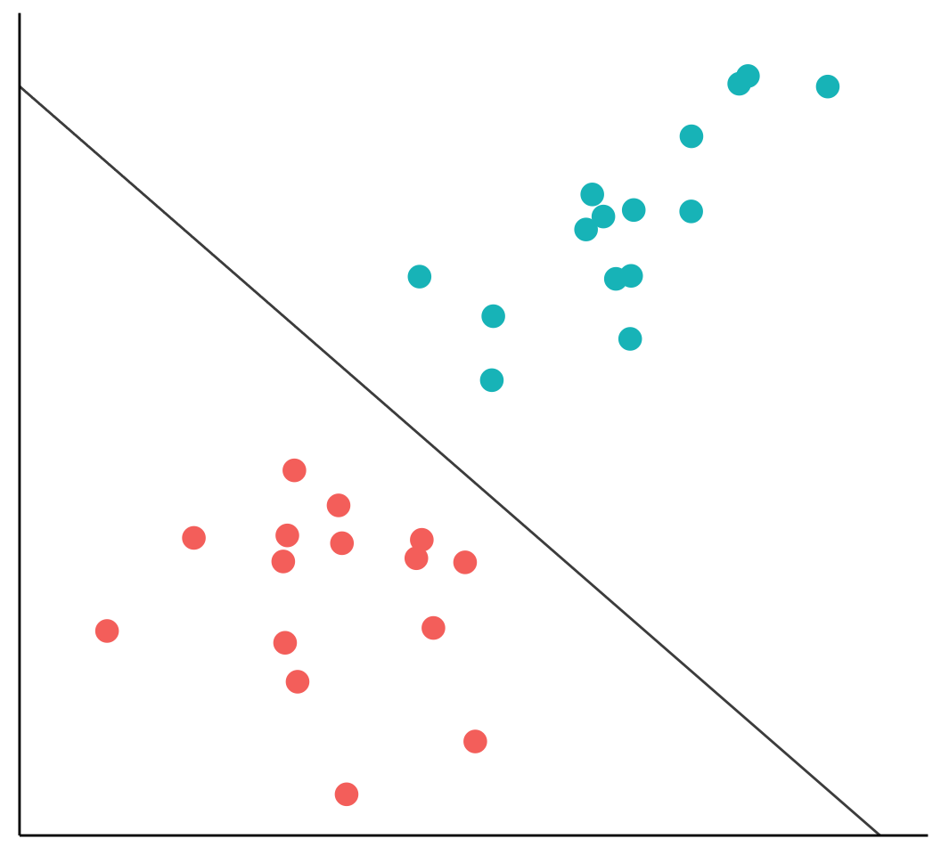
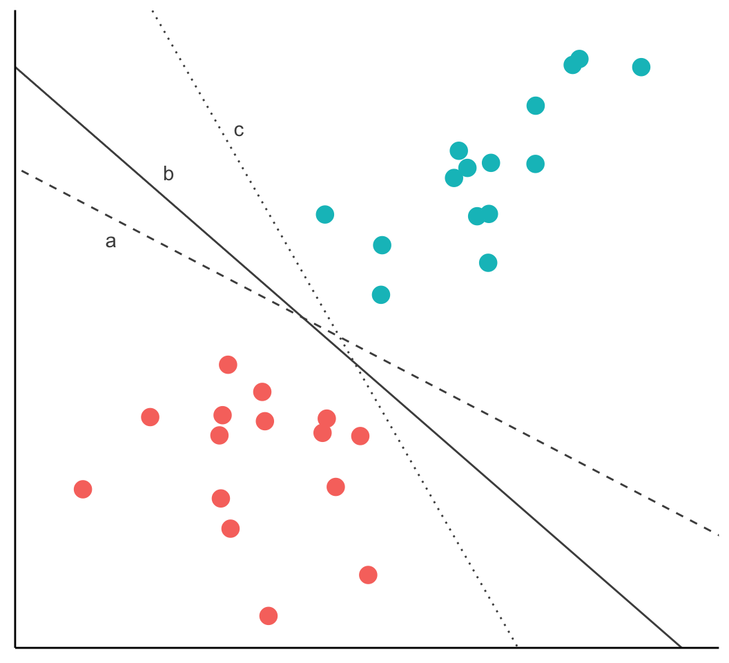
The task of the SVM algorithm is to identify a line that separates the two classes, but there os always more than one choice
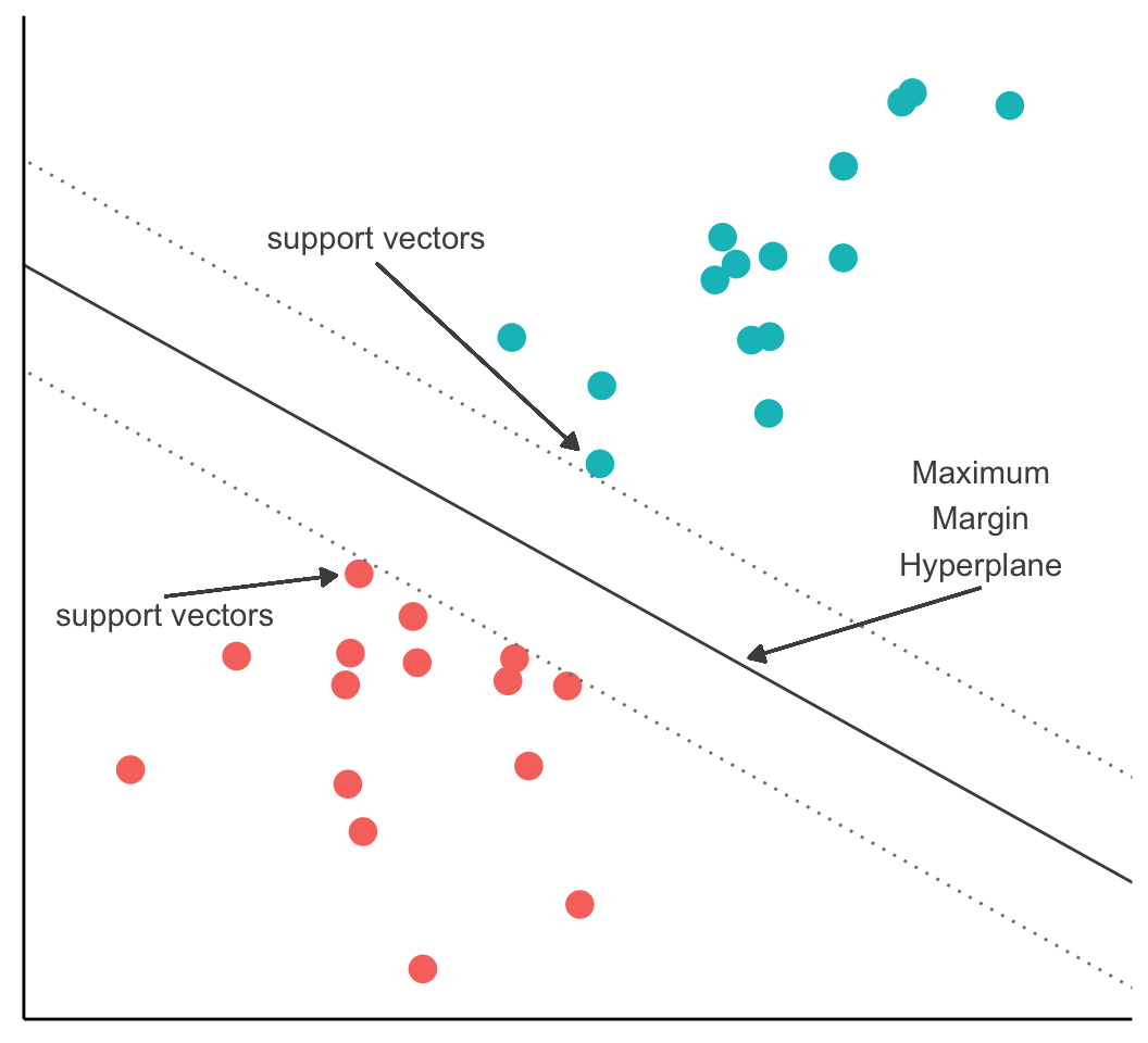
Therefore, the algorithm searches for the maximum margin hyperplane (MMH) that creates the greatest separation between the two classes, although any of the three lines separates the classes, the line that leads to the greatest separation will generalize best to new data
The support vectors are the points from each class that are closest to the MMH (each class must have at least on support vector)
The task of the SVM algorithm is to identify a line that separates the two classes, but there os always more than one choice
Therefore, the algorithm searches for the maximum margin hyperplane (MMH) that creates the greatest separation between the two classes, although any of the three lines separates the classes, the line that leads to the greatest separation will generalize best to new data
The support vectors are the points from each class that are closest to the MMH (each class must have at least on support vector)
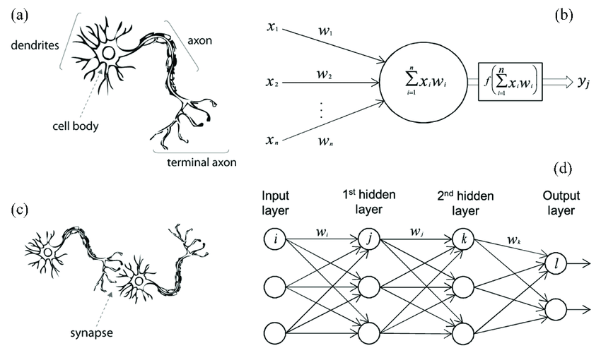
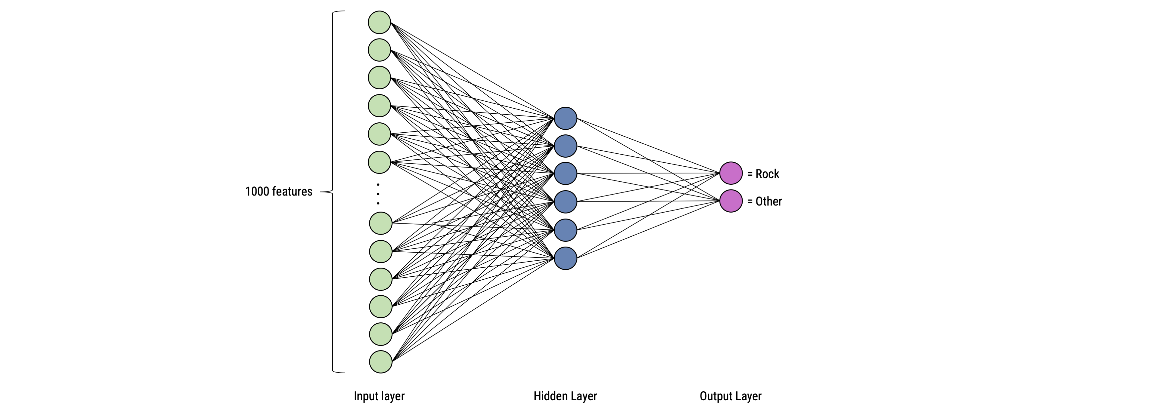
An artificial neural network (ANN) models the relationship between a set of input signals and an output signal using a model derived from our understanding of the human brain
Like a brain uses a network of interconnected cells called “neurons” (a) to provide fast learning capabilities, ANN uses a network of artificial neurons (b) to solves learning tasks
Source: Arthur Arnx/Medium
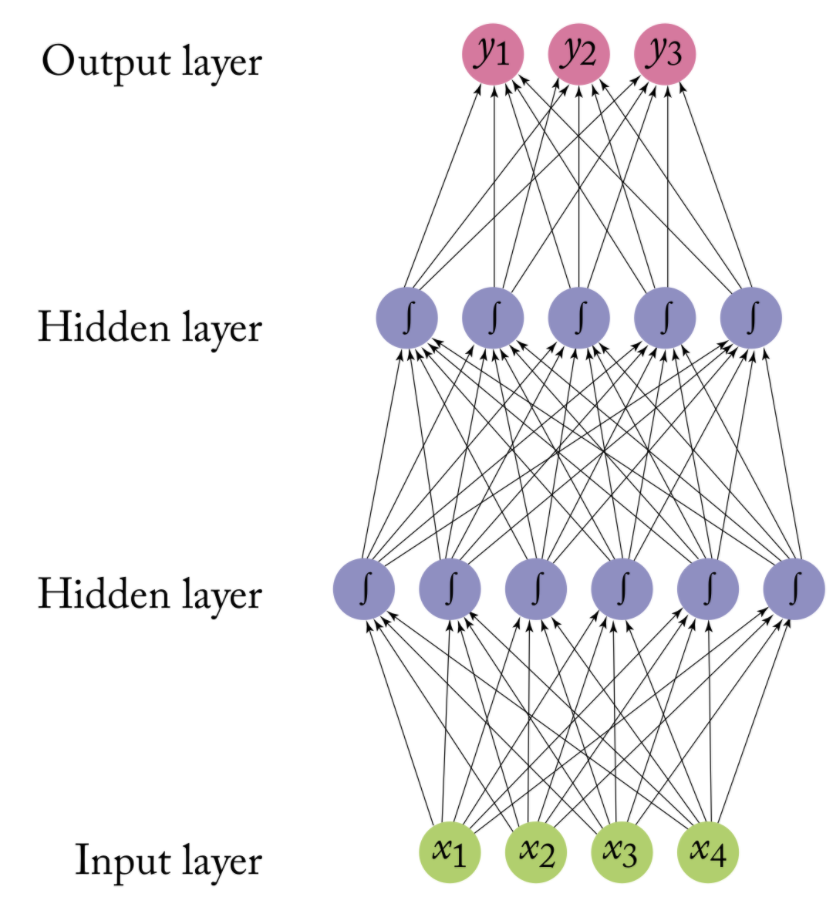
The operation of an ANN is straightforward:
In the simplest form, neurons on are stacked on top of one another and a neuron of colum n can only be connected to inputs from column n-1 and provide outputs to neurons in column n+1
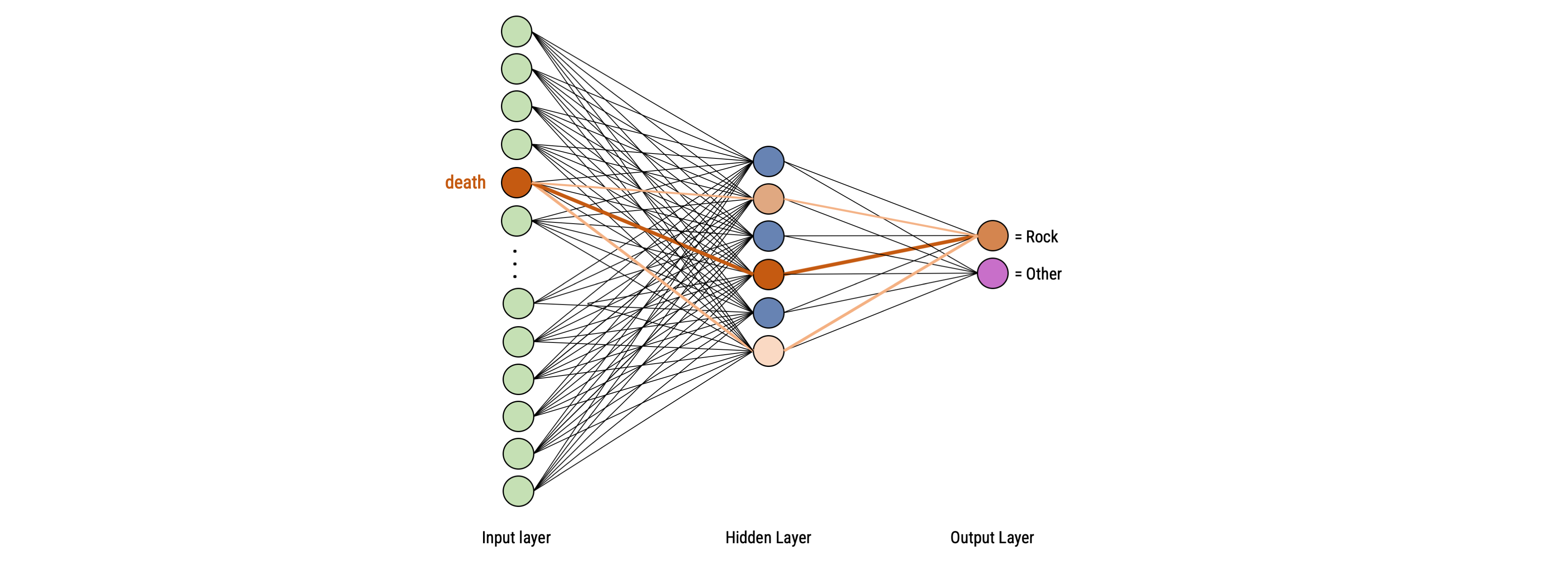
First, a neuron adds up the value of every neurons from the previous column it is connected to (here x1, x2, and x3)
This value is multiplied, before being added, by another variable called “weight” (w1, w2, w3): the strength of connection between two neurons
A bias value may be added (e.g., to regularize the network)
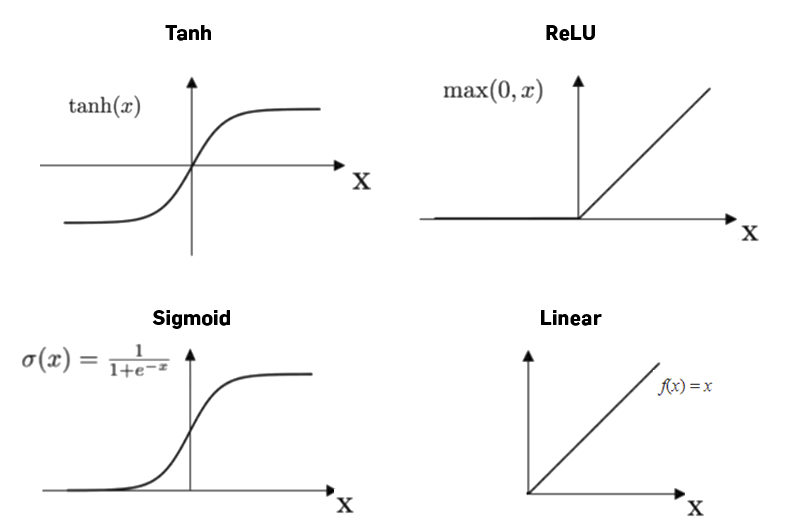
After all those summations, the neuron finally applies a function called activation function to the obtained value
Source: Arthur Arnx/Medium
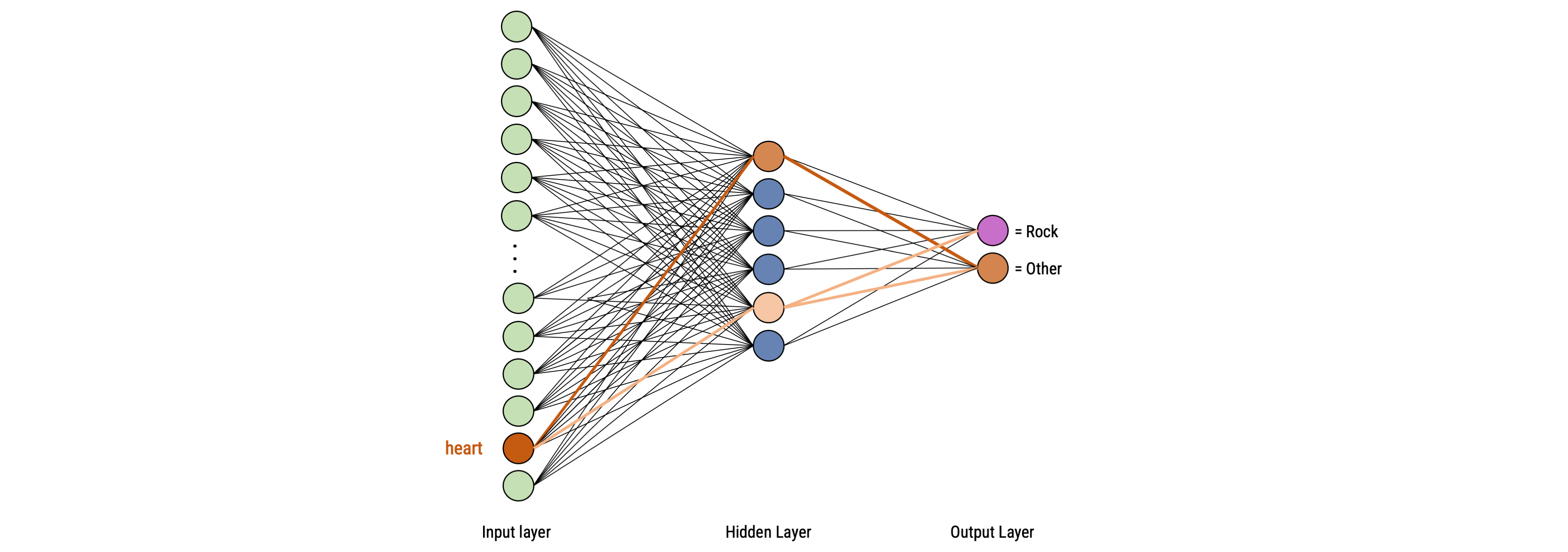
The activation function serves to turn the total value calculated to a number between 0 and 1
A threshold then defines at what value the function should “fire” the output to the next neuron (of course this can be probabilistic)
We can choose from different activation functions; which works best is sometimes hard to tell
 In a first try, the ANN randomly sets weights and thus can’t get the right output (except with luck)
If the (random) choice was a good one, actual parameters are kept and the next input is given. If the obtained output doesn’t match the desired output, the weights are changed.
To determine which weight is better to modify, a ANN uses backpropagation, which consists of “going back” on the neural network and inspect every connection to check how the output would behave according to a change on the weight
The learning rate thereby determines the speed a neural network will learn, i.e., how it will modify a weight (e.g., little by little or by bigger steps).
Learning rate and number of learning cycles (epochs) have to be set manually upfront!
A simple model with just inputs and outputs is called a perceptron
Despite its usefulness for many tasks, it cannot combine features
But we can add “hidden” layers (latent variables), creating a multilayer perceptron, which is able to process more complex inputs
Backpropagation is thus the way a neural network adjusts the weights of its connections (-> Can take a long time to find the right solutions)
Universal approximator: Neural Networks with single hidden layer can represent every continuous function!
# For replication purposes
set.seed(42)

# Specify multilayer perceptron
nnet_spec <-
  mlp(epochs = 400,          # <- times that algorithm will work through train set
      hidden_units = c(6),   # <- nodes in hidden units
      penalty = 0.01,        # <- regularization
      learn_rate = 0.2) |>   # <- shrinkage
  set_engine("brulee") |>    # <-- engine = R package
set_mode("classification")# For replication purposes
set.seed(42)
# Specify multilayer perceptron
nnet_spec <-
mlp(epochs = 400, # <- times that algorithm will work through train set
hidden_units = c(6), # <- nodes in hidden units
penalty = 0.01, # <- regularization
learn_rate = 0.2) |> # <- shrinkage
set_engine("brulee") |> # <-- engine = R package
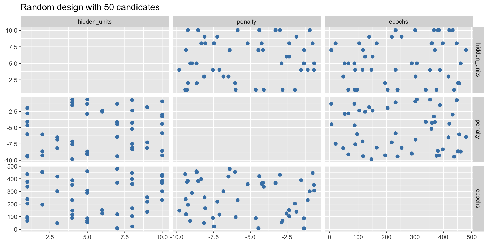
set_mode("classification")We can plot the random combinations to get an idea what they will cover
Bear in mind, such a grid search would be quite computationally intensive as 50 neural networks would need to be fitted!
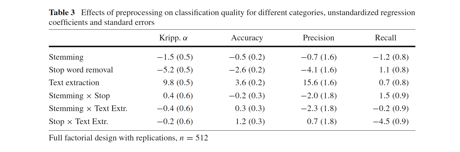
Scharkow ran a simple simulation study in which he systematically varied text preprocessing
The classifier was always Naive Bayes, below we see the average difference in performance
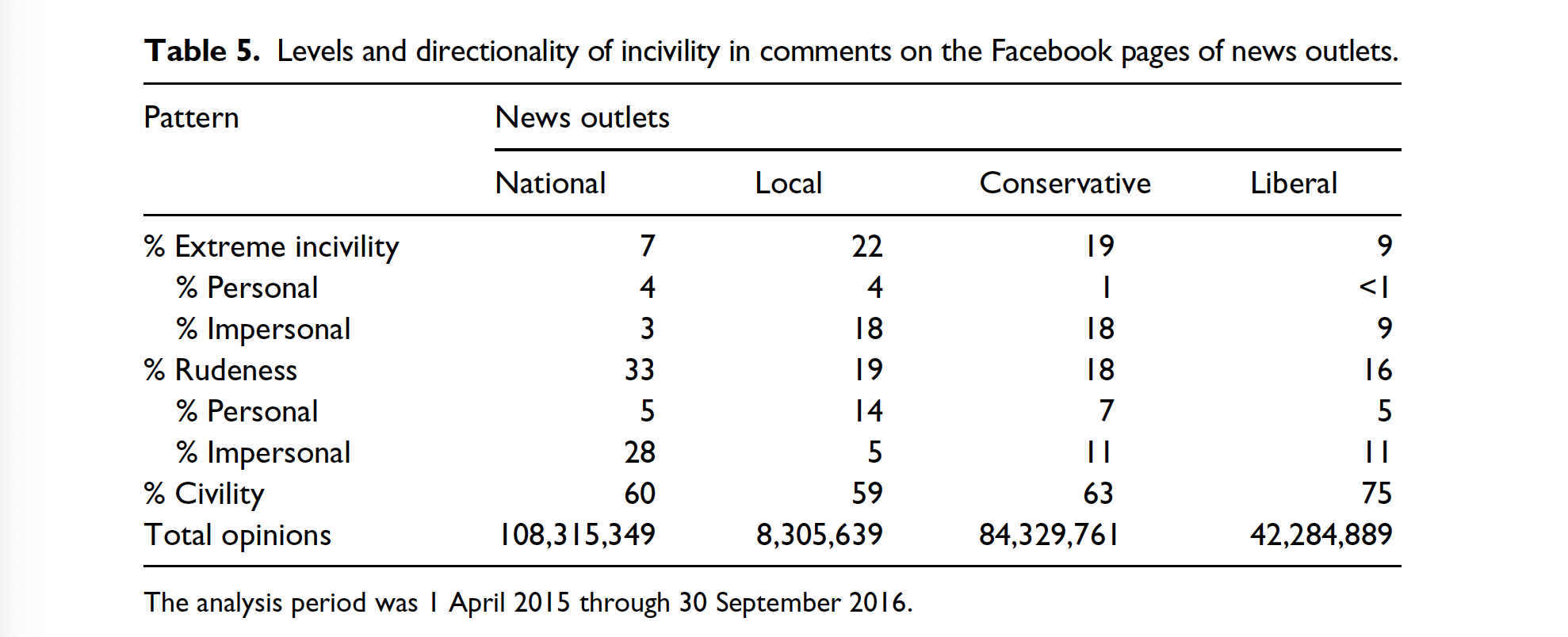
de León et al. (2021) explored how elections transform news sharing behaviour on Facebook
They investigated changes in news coverage and news sharing behaviour on Facebook
Employed a novel data set of news articles (N = 83,054) in Mexico
First coded 2,000 articles manually into topics (Politics, Crime and Disasters, Culture and Entertainment, Economic and Business, Sports, and Other), then used support vector machines to classify the rest

During periods of heightened political activity, both the publication and dissemination of political news increases
The gap between the news choices of journalists and consumers narrows, and increased political news sharing leading to a decrease in the sharing of other news.
Classic machine learning is a useful tool for generalizing from a sample
It is very useful to reduce the amount of manual coding needed
That said, the field has moved on and innovations are fast-paced these days:
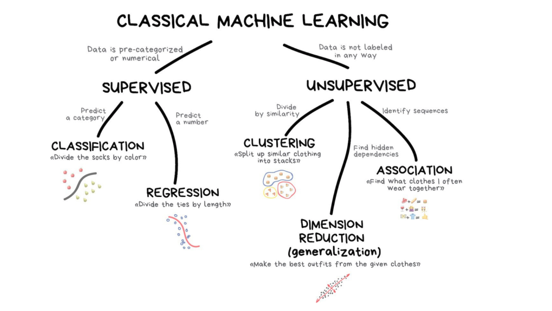
Describe the typical process used in supervised text classification.
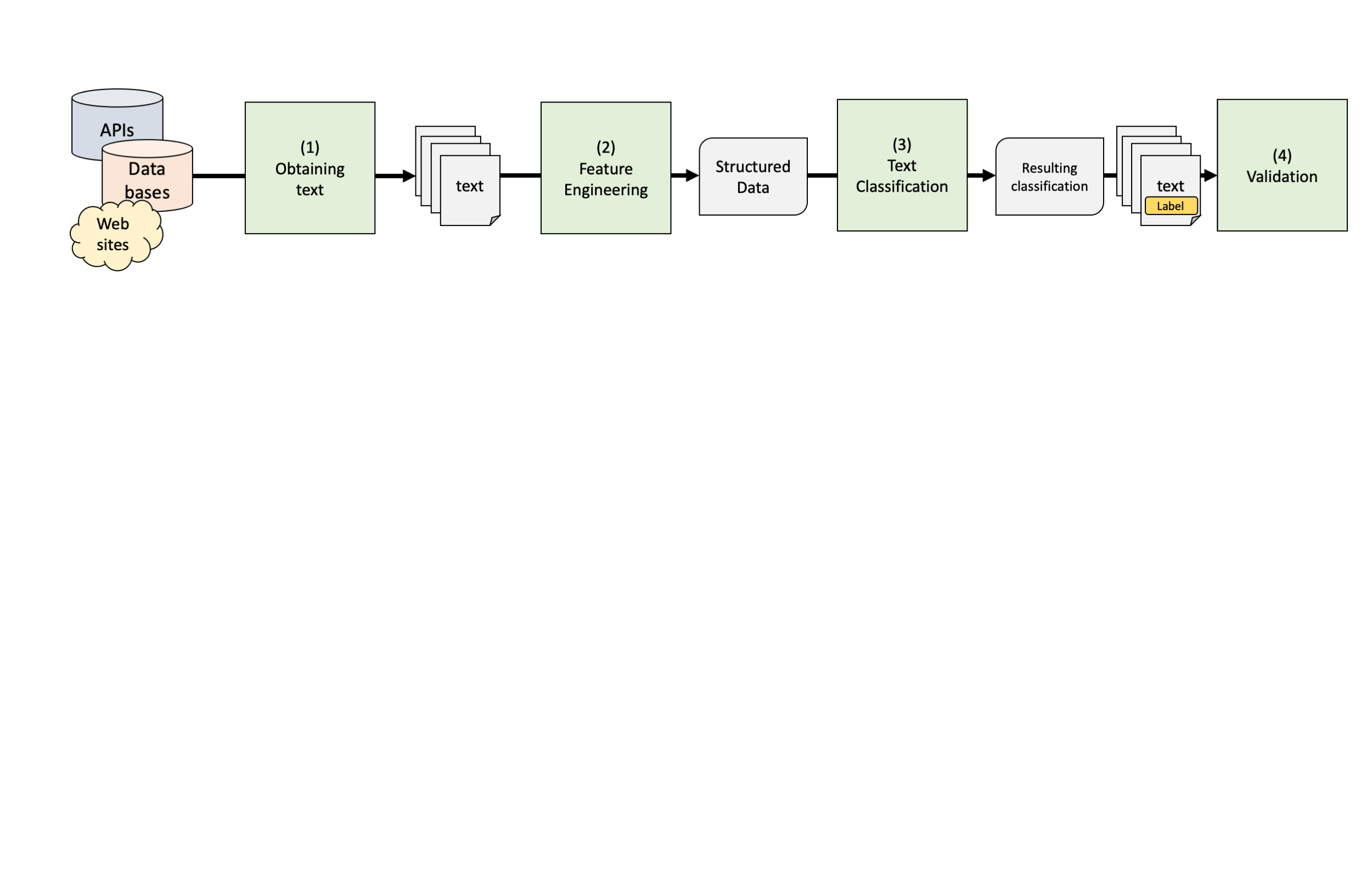
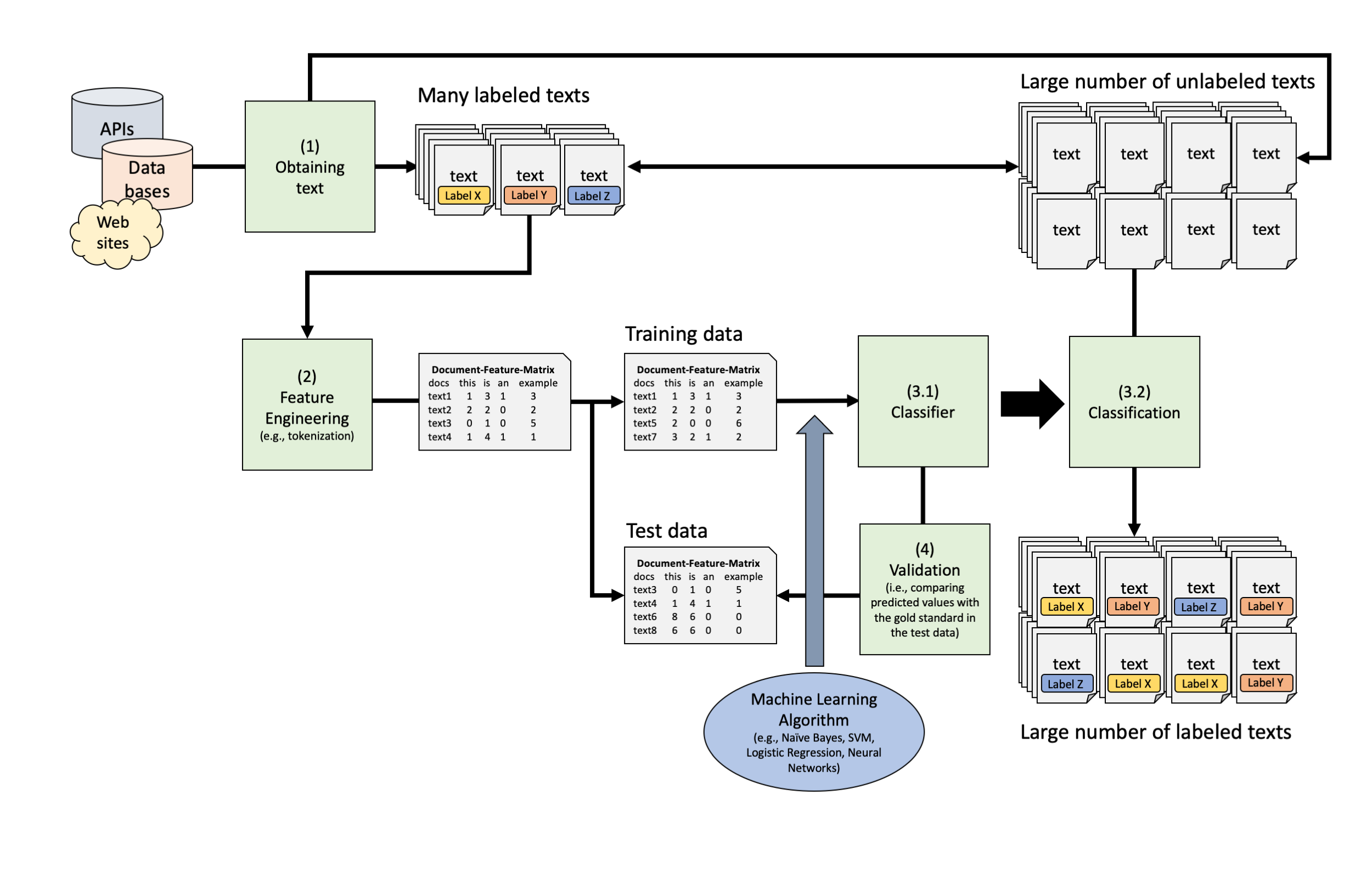
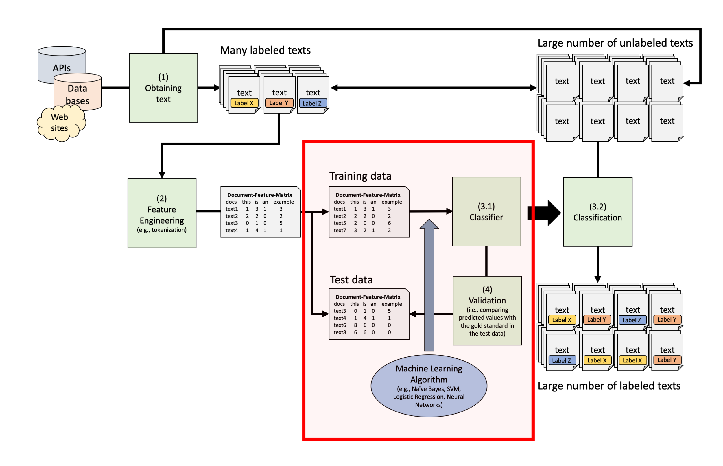
Any supervised machine learning procedure to analyze text usually contains at least 4 steps:
One has to manually code a small set of documents for whatever variable(s) you care about (e.g., topics, sentiment, source,…).
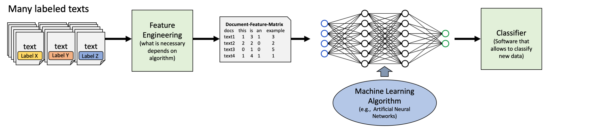
One has to train a machine learning model on the hand-coded /gold-standard data, using the variable as the outcome of interest and the text features of the documents as the predictors.
One has to evaluate the effectiveness of the machine learning model via cross-validation. This means one has to test the model test on new (held-out) data.
Once one has trained a model with sufficient predictive accuracy, precision and recall, one can apply the model to more documents that have never been hand-coded or use it for the purpose it was designed for (e.g., a spam filter detection software)
![]()