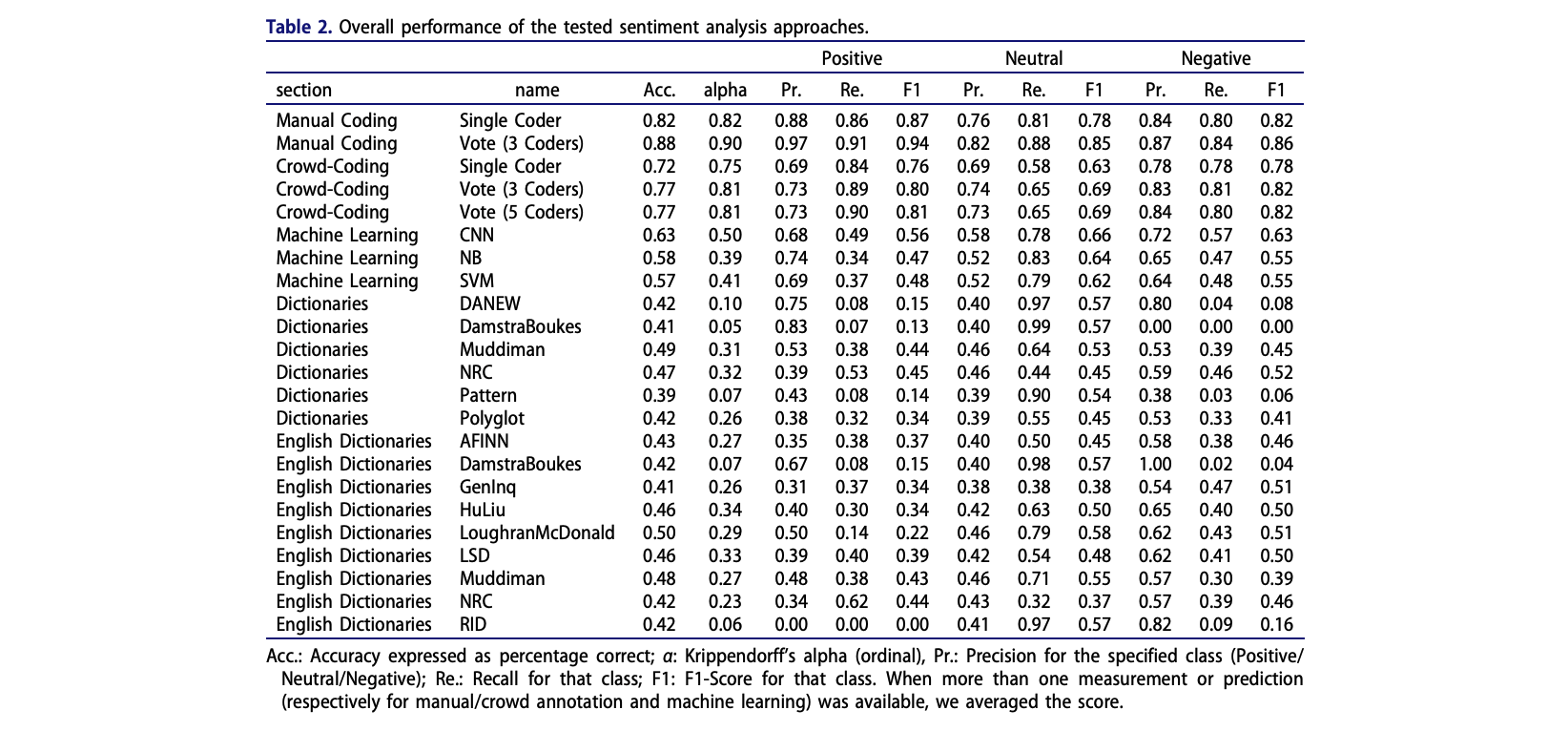
Main results
Week 3: Neural Networks and Word-Embeddings
Machine learning is the study of computer algorithms that can improve automatically through experience and by the use of data
Due to the “black box” nature of the algorithm’s operations, it is often seen as a form of artificial intelligence
Source: qlik
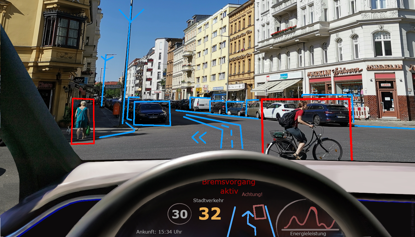 Successful machine learning in practical contexts:
What is Machine Learning?
1.1. Concepts and Principles
1.2. The General Machine Learning Pipeline
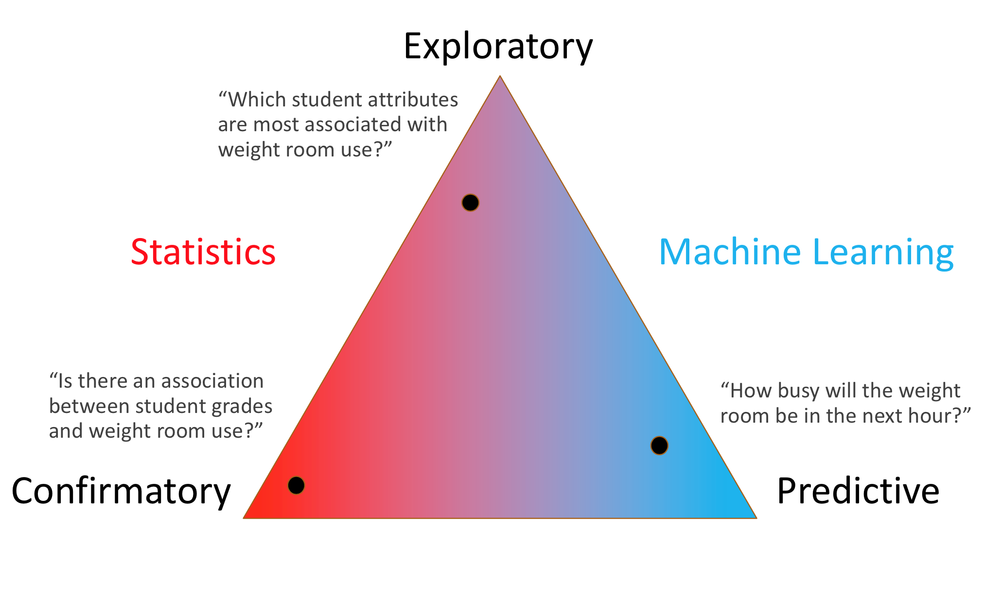
1.3. Difference between Statistics and Machine Learning
1.4. Over- vs. underfitting
1.5. Training vs. Testing
Text Classification with Artificial Neural Networks
2.1. Overview of classic ML algorithms
2.2. General Idea behind Neural Networks
2.3. How A Neural Network Works
2.4. How A Neural Network Learns
2.5. Example using Actual Data
More Complex Text Representations: Word-Embeddings
3.1. Basic Idea behind Vector-Representations
3.2. Similarity of Words and Texts
3.3. Using Pre-trained Word-Embeddings: GloVe
Text Classification with Word-Embeddings
4.1. Text Classification Pipeline with Word-Embeddings
4.2. Example with Actual Data
4.4. Fine-Tuning and Grid Search
Examples from the Literature
4.1. Incivility on Facebook (Su et al., 2018)
4.2. Electoral News Sharing (de León et al., 2021)
Summary and Conclusion
Understanding Supervised Machine Learning Approaches
In the previous lecture, we talked about deductive approaches (e.g., dictionary approaches)
These are deterministic and are based on a priori text theory
(e.g., happy → positive, hate → negative)
Yet, natural language is often ambiguous and a probabilistic coding may be better
Dictionary-based or generally rule-based approaches are not very similar to manual coding; a human being assesses much more than just a list of words
Inductive approaches promise to combine the scalability of automatic coding with the validity of manual coding
Machine learning, many people joke, is nothing but a fancy name for statistics.
There is some truth to this: the term “logistic regression” will sound familiar to both statisticians and machine learning practitioners.
Still, there are some differences between traditional statistical approaches and the machine learning approach, even if some of the same mathematical tools are used.
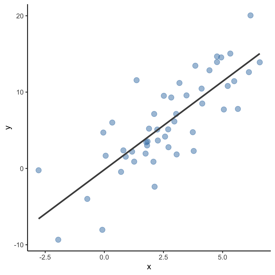
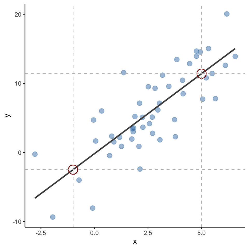
Is about understanding the relationship between one (or several) predictor(s) and an outcome variable
Learn \(f\) so you can predict \(y\) from \(x\):
x increases by 1 unit,y increases by 2.31 units.
Machine learning less about not understanding, but about maximizing prediction
A statistical model can be used to predict most likely \(y\) values based on new \(x\) data.
For example, despite not being in the data, \(x = -1\) should be \(y = -2.47\); \(x = 5\) should be \(y = 11.41\) based on the fitted line
In other words, machine learning doesn’t focus on explanation, but emphasizes prediction
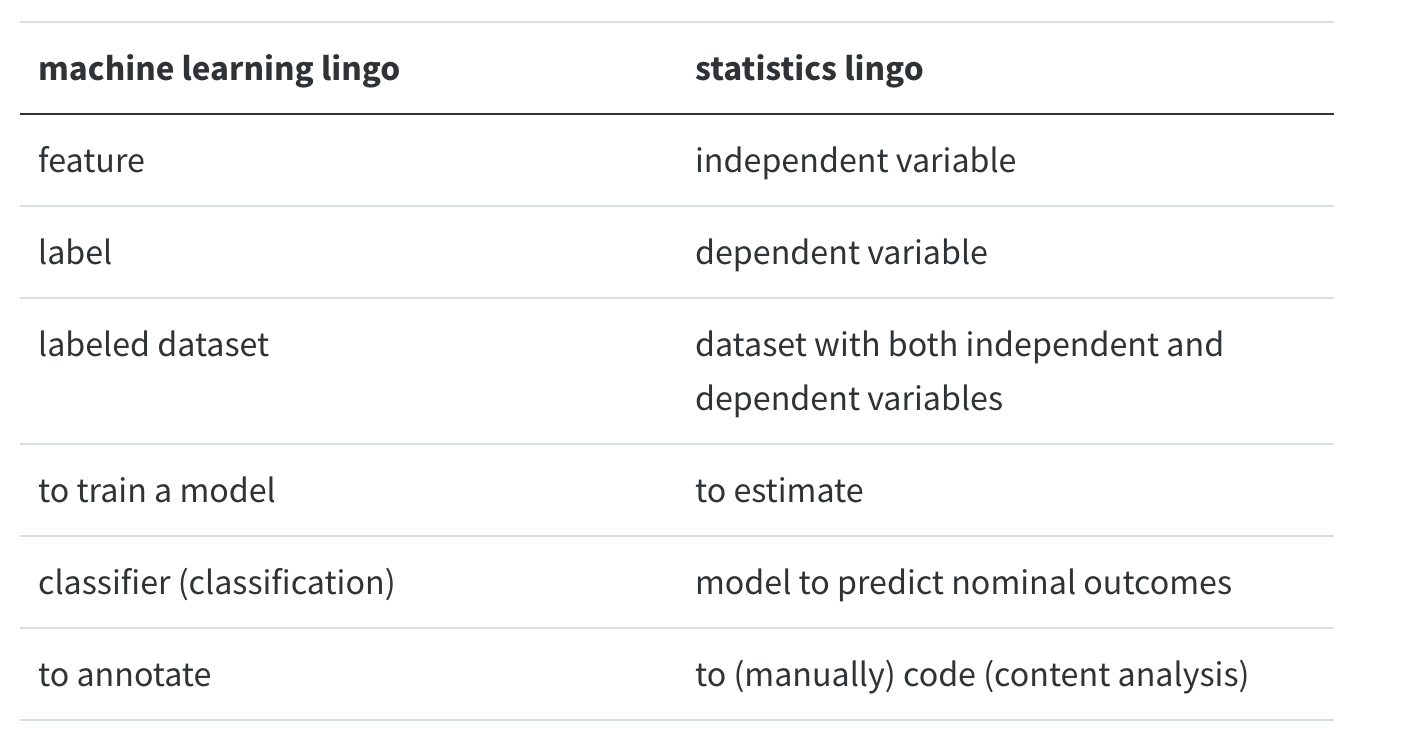
Goal of statistical modeling: explaining/understanding
Goal of machine learning: best possible prediction
Note: Machine learning models often have 1000’s of colinear independent variables and can have many latent variables!
Problem in Machine Learning: Sufficiently complex algorithms can predict all training data perfectly
But such an algorithm does not generalize to new data
Essentially, we want the model to have a good fit to the data, but we also want it to not optimize on things that are specific to the training data set
Let’s try exemplify over vs. underfit with some simulated data!
Regularization during fitting process
Out-of-sample validation
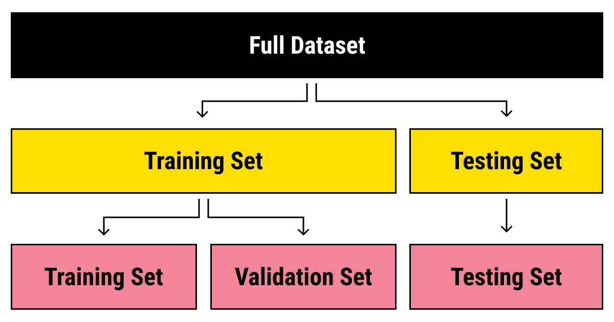
As models (almost) always overfit, performance on only training data is not a good indicator of the real quality of the classifier
The standard solution is to split the labeled data into a training and test data sets: We train the algorithm on one part and then evaluate its performance on the held-out part
Remember how we validated dictionary approaches?
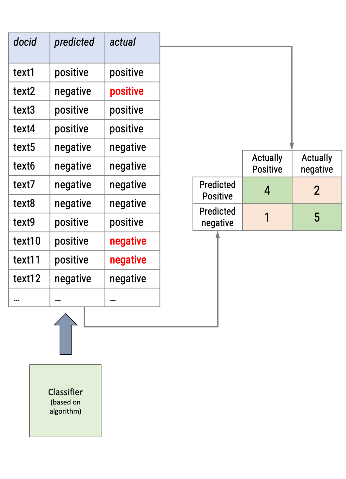
In supervised text classification, the procedure is similar:
Translating the Architecture of the Brain into Algorithmic Processing
→ In the following, we will focus primarily on neural networks as the most advanced algorithm in ML, but note that we could easily use other algorithms as well
# A tibble: 15,880 × 4
      id label            title                                                                                    text
   <dbl> <chr>            <chr>                                                                                    <chr>
 1     1 computer science Reconstructing Subject-Specific Effect Maps                                              "Rec…
 2     2 computer science Rotation Invariance Neural Network                                                       "Rot…
 3     5 computer science Comparative study of Discrete Wavelet Transforms and Wavelet Tensor Train decomposition… "Com…
 4     7 physics          On the rotation period and shape of the hyperbolic asteroid 1I/`Oumuamua (2017) U1 from… "On …
 5     8 physics          Adverse effects of polymer coating on heat transport at solid-liquid interface           "Adv…
 6     9 physics          SPH calculations of Mars-scale collisions: the role of the Equation of State, material … "SPH…
 7    11 computer science A global sensitivity analysis and reduced order models for hydraulically-fractured hori… "A g…
 8    12 physics          Role-separating ordering in social dilemmas controlled by topological frustration        "Rol…
 9    13 physics          Dynamics of exciton magnetic polarons in CdMnSe/CdMgSe quantum wells: the effect of sel… "Dyn…
10    14 computer science On Varieties of Ordered Automata                                                         "On …
# ℹ 15,870 more rowsThe data contains articles from computer science, physics, and statistics
Our goal is to find a neural network archtecture that can label abstracts with these disciplines sufficiently well
For the entire model fitting process, we are going to use the package tidymodels, which nicely intersects with the already known package tidytext
Here, we can use the functions initial_split to split our data set. The functions training and testing create the actual data sets from the splits.
library(tidymodels)

# Set seed to insure replicability
set.seed(42)

# Create initial split proporations
split <- initial_split(science_data, prop = .90)

# Create training and test data
train_data <- training(split)
test_data <- testing(split)

# Check
tibble(dataset = c("training", "testing"),
       n_songs = c(nrow(train_data), nrow(test_data)))
Classic machine learning models require a numerical representation of text (e.g., document-feature matrix)
They further need the outcome variable that they should predict
All text-preprocessing steps (e.g., stopword removal, stemming, frequency trimming,etc.) may change the performance, but no clear rules on what works and what does not
Only solution: Trial and error!

library(tidytext)

# Text Preprocessing
dfm_train <- train_data |>
  unnest_tokens(word, text) |>                     # <-- Tokenization
  anti_join(stop_words) |>                         # <-- Remove stop words
  group_by(id, word) |>                            # <-- group by text and word
  summarize(n = n()) |>                            # <-- count word frequencies
  cast_dfm(document = id, term = word,  value = n) # <-- create DFM

# Check
dfm_train |>
  head()
Document-feature matrix of: 6 documents, 48,379 features (99.87% sparse) and 0 docvars.
features
docs accuracy ad adni aims algorithm alterations alzheimer's amyloid analyses analyzing
1 1 1 3 1 1 1 2 1 1 1
2 0 0 0 0 0 0 0 0 0 0
5 1 0 0 0 0 0 0 0 0 0
7 0 0 0 0 0 0 0 0 0 0
8 0 0 0 0 0 0 0 0 0 0
9 0 0 0 0 0 0 0 0 0 0
[ reached max_nfeat ... 48,369 more features ]library(textrecipes)
# Create recipe for text preprocessing
rec <- recipe(label ~ text, data = science_data) |>
step_tokenize(text, options = list(strip_punct = T, strip_numeric = T)) |> # <-- Tokenization
step_stopwords(text, language = "en") |> # <-- Remove stop words
step_tf(all_predictors()) # <-- Create DFM
# "Bake" (check) based on recipe to see text preprocessing
rec |>
prep(train_data) |>
bake(new_data=NULL)# A tibble: 14,292 × 44,333
label tf_text__aster tf_text__b tf_text__c tf_text__catalogue tf_text__d tf_text__e tf_text__f tf_text__g tf_text__h
<fct> <int> <int> <int> <int> <int> <int> <int> <int> <int>
1 stati… 0 0 0 0 0 0 0 0 0
2 physi… 0 0 0 0 0 0 0 0 0
3 physi… 0 0 0 0 0 0 0 0 0
4 compu… 0 0 0 0 0 0 0 0 0
5 compu… 0 0 0 0 0 0 0 0 0
6 compu… 0 0 0 0 1 0 0 0 0
7 compu… 0 0 0 0 0 0 0 0 0
8 physi… 0 0 0 0 0 0 0 0 0
9 physi… 0 0 0 0 0 0 0 0 0
10 compu… 0 0 0 0 0 0 0 0 0
# ℹ 14,282 more rows
# ℹ 44,323 more variables: tf_text__i <int>, tf_text__j <int>, tf_text__k <int>, tf_text__m <int>, tf_text__n <int>,
# tf_text__p <int>, tf_text__q <int>, tf_text__r <int>, tf_text__s <int>, tf_text__svd <int>, tf_text__t <int>,
# tf_text__u <int>, tf_text__v <int>, tf_text__x <int>, tf_text__y <int>, tf_text__z <int>, tf_text_0.0001s <int>,
# tf_text_0.031mj <int>, tf_text_0.05dex <int>, tf_text_0.12v <int>, tf_text_0.18um <int>, tf_text_0.1c <int>,
# tf_text_0.1dex <int>, tf_text_0.254r <int>, tf_text_0.2c <int>, tf_text_0.2db <int>, tf_text_0.2l <int>,
# tf_text_0.2r_ <int>, tf_text_0.3a <int>, tf_text_0.3t_ <int>, tf_text_0.4gyr <int>, tf_text_0.4k <int>, …The collection tidymodels contains a variety of packages that facilitates and streamlines machine learning in R
The basic procedure is the following:

# Load specific support library
library(textrecipes)

# Create recipe
rec <- recipe(label ~ text, data = science_data) |>               # <-- predict binary_genre by text
  step_tokenize(text, options = list(strip_punct = T,             # <-- tokenize, remove punctuation
                                     strip_numeric = T)) |>       # <-- remove numbers
  step_stopwords(text, language = "en") |>                        # <-- remove stopwords
step_tokenfilter(text, min_times = 20, max_tokens = 1000) # <-- filter out rare words and use only top 1000 # Load specific support library
library(textrecipes)
# Create recipe
rec <- recipe(label ~ text, data = science_data) |> # <-- predict binary_genre by text
step_tokenize(text, options = list(strip_punct = T, # <-- tokenize, remove punctuation
strip_numeric = T)) |> # <-- remove numbers
step_stopwords(text, language = "en") |> # <-- remove stopwords
step_tokenfilter(text, min_times = 20, max_tokens = 1000) |> # <-- filter out rare words and use only top 1000
step_tf(all_predictors()) # <-- create document-feature matrix# Load specific support library
library(textrecipes)
# Create recipe
rec <- recipe(label ~ text, data = science_data) |> # <-- predict binary_genre by text
step_tokenize(text, options = list(strip_punct = T, # <-- tokenize, remove punctuation
strip_numeric = T)) |> # <-- remove numbers
step_stopwords(text, language = "en") |> # <-- remove stopwords
step_tokenfilter(text, min_times = 20, max_tokens = 1000) |> # <-- filter out rare words and use only top 1000
step_tf(all_predictors()) # <-- create document-feature matrix
# Small adaption to the recipe (for SVM and neural networks)
rec_norm <- rec |>
step_normalize(all_predictors()) An artificial neural network models the relationship between a set of input signals and an output signal using a model derived from our understanding of the human brain
Like a brain uses a network of interconnected cells called “neurons” (a) to provide fast learning capabilities, a neural network uses a network of artificial neurons (b) to solves learning tasks
Source: Arthur Arnx/Medium
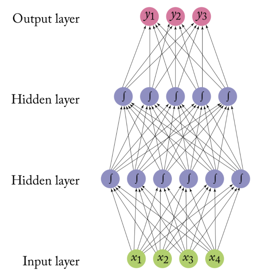
The operation of an artificial neural network is straightforward:
Neurons are stacked on top of one another and a neuron of colum n can only be connected to inputs from column n-1 and provide outputs to neurons in column n+1
In other words, input data are passed through layered transformations until an output is reached
First, the value of each input neuron is multiplied by so-called “weight” (w1, w2, w3), which could be regarded as the strength of connection between two neurons
Second, the neuron adds up the values of every input neuron from the previous column it is connected to (here x1, x2, and x3)
Third, a bias value may be added (e.g., to regularize the network)
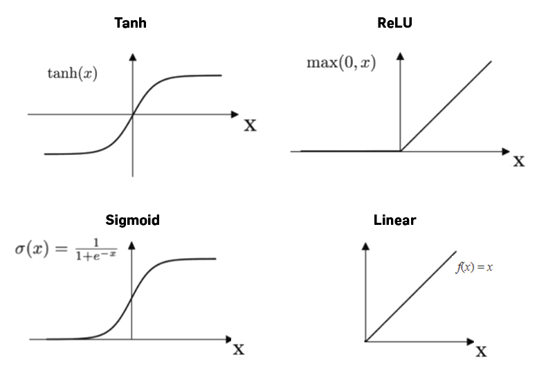
After all those summations, the neuron finally applies a function called “activation function” to the obtained value
Source: Arthur Arnx/Medium
The activation function serves to turn the total value calculated to a number between 0 and 1
A threshold then defines at what value the function should “fire” the output to the next neuron (of course this can be probabilistic)
We can choose from different activation functions; which works best is sometimes hard to tell
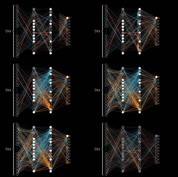 In a first try, the neural network randomly sets weights and thus can’t get the right output (except with luck)
If the random choice was a good one, actual parameters are kept and the next input is given. If the obtained output doesn’t match the desired output, the weights are changed
To determine which weight is better to modify, a neural network uses backpropagation, which consists of “going back” on the neural network and inspect every connection to check how the output would behave according to a change on the weight
The learning rate thereby determines the speed a neural network will learn, i.e., how it will modify a weight (e.g., little by little or by bigger steps).
Learning rate and number of learning cycles (so-called epochs) have to be set manually upfront!
It is hard to imagine how the network has learned that a certain combination of words corresponds to a certain label.
In fact, we can only speculate that it might capture certain meaning by co-occurence of words, e.g., that certain words are representing machine learning and machine learning, in turn, is most likely to be within “computer science”
# For replication purposes
set.seed(42)

# Specify multilayer perceptron
nnet_spec <-
  mlp(epochs = 400,          # <- times that algorithm will work through train set
      hidden_units = c(6),   # <- nodes in hidden units
      penalty = 0.01,        # <- regularization
      learn_rate = 0.2) |>   # <- shrinkage
  set_engine("brulee") |>    # <- engine = R package
  set_mode("classification")

# Create workflow
ann_workflow <- workflow() |>
  add_recipe(rec_norm) |>    # Use updated recipe with normalization
add_model(nnet_spec)# For replication purposes
set.seed(42)
# Specify multilayer perceptron
nnet_spec <-
mlp(epochs = 400, # <- times that algorithm will work through train set
hidden_units = c(6), # <- nodes in hidden units
penalty = 0.01, # <- regularization
learn_rate = 0.2) |> # <- shrinkage
set_engine("brulee") |> # <- engine = R package
set_mode("classification")
# Create workflow
ann_workflow <- workflow() |>
add_recipe(rec_norm) |> # Use updated recipe with normalization
add_model(nnet_spec)
# Fit model
m_ann <- fit(ann_workflow, train_data)# Predict outcome in test data
predict_ann <- predict(m_ann, new_data = test_data) %>%
bind_cols(test_data) |>
mutate(truth = factor(label)) |>
select(id, predicted = .pred_class, truth, title)
# Check
predict_ann |>
head(n = 4)# A tibble: 4 × 4
id predicted truth title
<dbl> <fct> <fct> <chr>
1 31 computer science computer science mixup: Beyond Empirical Risk Minimiza…
2 35 computer science computer science Deep Neural Network Optimized to Resi…
3 48 computer science computer science Wehrl Entropy Based Quantification of…
4 55 computer science computer science An Effective Framework for Constructi…tidymodels, we have to define a set of measures that we want to compute based on the predictions in the test set.We then can inspect the confusion matrix
We see here that it does get a lot of articles right, but there are also some false positives and false negatives
With tidymodels, we can very easily use a different algorithm.
Because we already set up a recipe that works with Support Vector Machines, the only thing we have to do is update the workflow and add the new model
library(LiblineaR)

# Updating the workflow
svm_workflow <- workflow() |>
  add_recipe(rec_norm) |>                         # <-- Recipe remains the same!
  add_model(svm_linear(mode = "classification",   # <-- We just add a new model (e.g Support Vector Machines)
                     engine = "LiblineaR"))

# Fitting the SVM model
m_svm <- fit(svm_workflow, data = train_data)# Predict test data
predict_svm <- predict(m_svm, new_data=test_data) |>
bind_cols(test_data) |>
mutate(truth = factor(label)) |>
select(id, predicted = .pred_class, truth, title)
# Combine predict data from SVM and neural network
bind_rows(
# Compute class_metrics for SVM
predict_svm |>
class_metrics(truth=truth, estimate=predicted) |>
mutate(algorithm = "support vector machines"),
# Compute class_metrics for NN
predict_ann |>
class_metrics(truth=truth, estimate=predicted) |>
mutate(algorithm = "neural network")) |>
# Plot comparison
ggplot(aes(x = .metric, y = .estimate,
fill = algorithm)) +
geom_col(position=position_dodge(), alpha=.5) +
geom_text(aes(label = round(.estimate, 3)),
position = position_dodge(width=1)) +
ylim(0, 1) +
coord_flip() +
scale_fill_brewer(palette = "Dark2") +
theme_minimal(base_size = 18) +
theme(legend.position = "bottom") +
labs(y = "Performance Score", x = "", fill = "")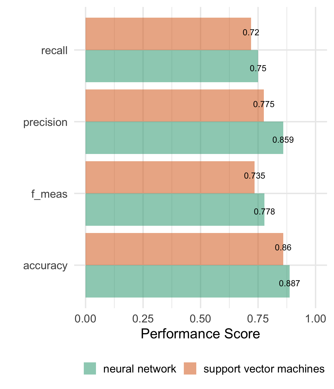
More Complex Text Representations
Computers don’t read text, they only can deal with numbers
For this reason, so far, we tokenized our texts (e.g., in words) and summarized their frequency across texts to create a document-feature matrix within the bag-of-words model
Such a text representation has some issues:
Word embeddings are a “learned” type of word representation that allows words with similar meaning to have a similar representation via a k-dimensional vector space
The first core idea behind word embeddings is that the meaning of a word can be expressed using a relatively small embedding vector, generally consisting of around 300 numbers which can be interpreted as dimensions of meaning
The second core idea is that these embedding vectors can be derived by scanning the context of each word in millions and millions of documents.
This means that words that are used in similar ways in the training data result in similar representations, thereby capturing their similar meaning.
All word embedding methods learn a real-valued vector representation for a predefined fixed-sized vocabulary from a corpus of text:
Via an embedding layer in a neural network designed for a particular downstream task
Learning word embeddings using a shallow neural network and context windows (e.g., word2vec)
Learning word embeddings by aggregating global word-word co-occurrence matrix (e.g., GloVe)
glove_fn = "glove.6B.50d.10k.w2v.txt"
url = glue::glue("https://cssbook.net/d/{glove_fn}")
if (!file.exists(glove_fn))
    download.file(url, glove_fn)

# Data wrangling
wv_tibble <- read_delim(glove_fn, skip=1, delim=" ", quote="",
    col_names = c("word", paste0("d", 1:50)))

# 10 highest scoring words on dimension 1
wv_tibble |>
  arrange(-d1) |> head()
# A tibble: 6 × 51
word d1 d2 d3 d4 d5 d6 d7 d8 d9 d10
<chr> <dbl> <dbl> <dbl> <dbl> <dbl> <dbl> <dbl> <dbl> <dbl> <dbl>
1 airbus 2.60 -0.536 0.414 0.339 -0.0510 0.848 -0.722 -0.361 0.869 -0.731
2 space… 2.52 0.744 1.66 0.0591 -0.252 -0.243 -0.594 -0.417 0.460 -0.124
3 fiat 2.29 -1.15 0.488 0.518 0.312 -0.132 0.0520 -0.661 -0.859 0.263
4 naples 2.27 -0.106 -1.27 -0.0932 -0.437 -1.18 -0.0858 0.469 -1.08 -0.549
5 di 2.24 -0.603 -1.47 0.354 0.244 -1.09 0.357 -0.331 -0.564 0.428
6 planes 2.20 -0.831 1.34 -0.348 -0.209 -0.282 -0.824 -0.481 0.211 -0.748
# ℹ 40 more variables: d11 <dbl>, d12 <dbl>, d13 <dbl>, d14 <dbl>, d15 <dbl>,
# d16 <dbl>, d17 <dbl>, d18 <dbl>, d19 <dbl>, d20 <dbl>, d21 <dbl>,
# d22 <dbl>, d23 <dbl>, d24 <dbl>, d25 <dbl>, d26 <dbl>, d27 <dbl>,
# d28 <dbl>, d29 <dbl>, d30 <dbl>, d31 <dbl>, d32 <dbl>, d33 <dbl>,
# d34 <dbl>, d35 <dbl>, d36 <dbl>, d37 <dbl>, d38 <dbl>, d39 <dbl>,
# d40 <dbl>, d41 <dbl>, d42 <dbl>, d43 <dbl>, d44 <dbl>, d45 <dbl>,
# d46 <dbl>, d47 <dbl>, d48 <dbl>, d49 <dbl>, d50 <dbl>With word-embeddings, we can compute similarity scores for word pairs, which proves the “encoding of meaning” in word-embeddings:
wv <- as.matrix(wv_tibble[-1])
rownames(wv) <- wv_tibble$word
wv <- wv / sqrt(rowSums(wv^2))
wvector <- function(wv, word) wv[word,,drop=F]
wv_similar <- function(wv, target, n=5) {
  similarities = wv %*% t(target)
  similarities |>
    as_tibble(rownames = "word") |>
    rename(similarity=2) |>
    arrange(-similarity) |>
    head(n=n)
}But we can also generalize word embeddings to entire sentences (or even texts):
library(ccsamsterdamR)

# Example sentences
movies <- tibble(sentences = c("This movie is great, I loved it.",
                               "The film was fantastic, a real treat!",
                               "I did not like this movie, it was not great.",
                               "Today, I went to the cinema and watched a movie",
                               "I had pizza for lunch.",
                               "Sometimes, when I read a book, I get completely lost."))

# Get embeddings from a sentence transformer
movie_embeddings <- hf_embeddings(txt = movies$sentences)

# Each text has now 384 values
movie_embeddings
# A tibble: 6 × 384
V1 V2 V3 V4 V5 V6 V7 V8 V9 V10 V11 V12 V13
<dbl> <dbl> <dbl> <dbl> <dbl> <dbl> <dbl> <dbl> <dbl> <dbl> <dbl> <dbl> <dbl>
1 -0.0875 -0.0156 -0.0380 -0.0586 -0.0842 0.0164 -0.0222 0.0451 0.0449 -0.00546 -0.0115 -0.00166 0.00575
2 -0.0544 0.0381 -0.0443 -0.0111 -0.0464 -0.00760 -0.0523 0.0173 -0.0725 -0.0432 0.0206 0.00903 0.0223
3 -0.0838 0.0135 -0.0938 -0.0351 -0.0848 -0.0424 -0.00107 0.0537 0.0559 -0.0729 0.0153 0.0359 0.0396
4 -0.0442 0.00655 0.0754 -0.0341 0.0637 0.00674 0.0993 -0.0369 0.0752 -0.0405 0.0222 0.0284 -0.0243
5 -0.0257 0.0440 0.0407 0.00391 -0.0818 -0.0621 0.0836 -0.0138 -0.101 -0.0757 0.0882 -0.0530 0.0351
6 0.0207 0.00907 -0.0388 0.0717 0.0419 0.0419 0.0267 0.0685 0.0879 -0.0125 0.0281 0.0503 -0.0437
# ℹ 371 more variables: V14 <dbl>, V15 <dbl>, V16 <dbl>, V17 <dbl>, V18 <dbl>, V19 <dbl>, V20 <dbl>, V21 <dbl>,
# V22 <dbl>, V23 <dbl>, V24 <dbl>, V25 <dbl>, V26 <dbl>, V27 <dbl>, V28 <dbl>, V29 <dbl>, V30 <dbl>, V31 <dbl>,
# V32 <dbl>, V33 <dbl>, V34 <dbl>, V35 <dbl>, V36 <dbl>, V37 <dbl>, V38 <dbl>, V39 <dbl>, V40 <dbl>, V41 <dbl>,
# V42 <dbl>, V43 <dbl>, V44 <dbl>, V45 <dbl>, V46 <dbl>, V47 <dbl>, V48 <dbl>, V49 <dbl>, V50 <dbl>, V51 <dbl>,
# V52 <dbl>, V53 <dbl>, V54 <dbl>, V55 <dbl>, V56 <dbl>, V57 <dbl>, V58 <dbl>, V59 <dbl>, V60 <dbl>, V61 <dbl>,
# V62 <dbl>, V63 <dbl>, V64 <dbl>, V65 <dbl>, V66 <dbl>, V67 <dbl>, V68 <dbl>, V69 <dbl>, V70 <dbl>, V71 <dbl>,
# V72 <dbl>, V73 <dbl>, V74 <dbl>, V75 <dbl>, V76 <dbl>, V77 <dbl>, V78 <dbl>, V79 <dbl>, V80 <dbl>, V81 <dbl>, …We can see that text 2 is most similar to text 1: Both express a very similar sentiment, just with different words (“great” ≈ “fantastic”; “I loved it” ≈ “A real treat”)
Text 2 is still similar to text 3 (after all it is about movies), but less so compared to text 1 (“fantastic” is the opposite of “not great”)
Text 4 still shares similarities (the context is the cinema/watching movies), but text 5 is very different as it doesn’t contain similar words and is not about similar things (except “I”).
Text 5 is very dissimilar to the others.
# Similarity between 2nd and the other sentences
movies |>
  mutate(similarity = as.matrix(movie_embeddings) %*% t(as.matrix(movie_embeddings)[2,, drop = F])) |>
  arrange(-similarity)
# A tibble: 6 × 2
sentences similarity[,1]
<chr> <dbl>
1 The film was fantastic, a real treat! 1.00
2 This movie is great, I loved it. 0.646
3 I did not like this movie, it was not great. 0.513
4 Today, I went to the cinema and watched a movie 0.372
5 I had pizza for lunch. 0.132
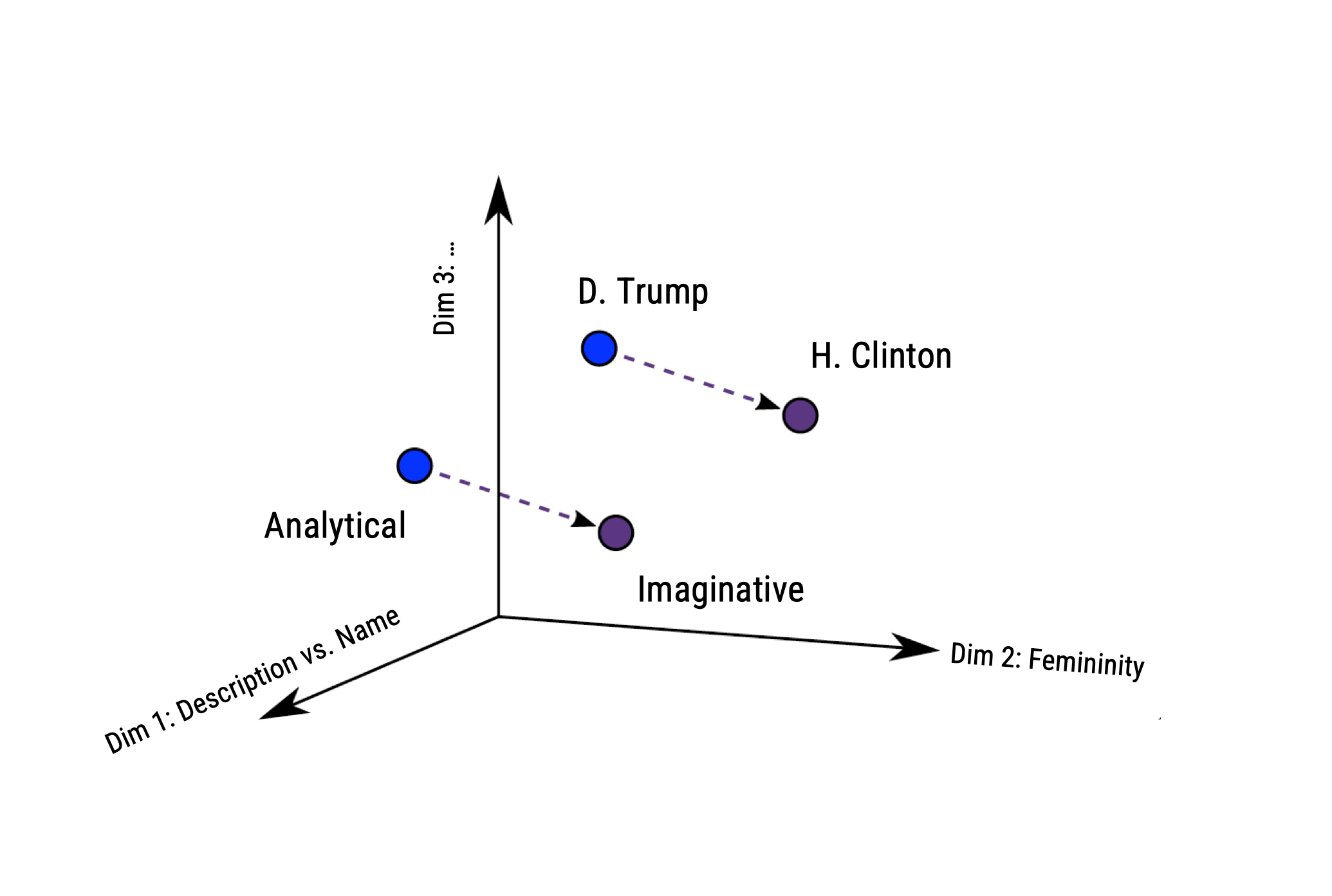
6 Sometimes, when I read a book, I get completely lost. 0.0939Based on vector-based computations, we can analyse semantic relationships
This is a quite common approach by now in research on gender and other types of stereotypes
Source: https://developers.google.com
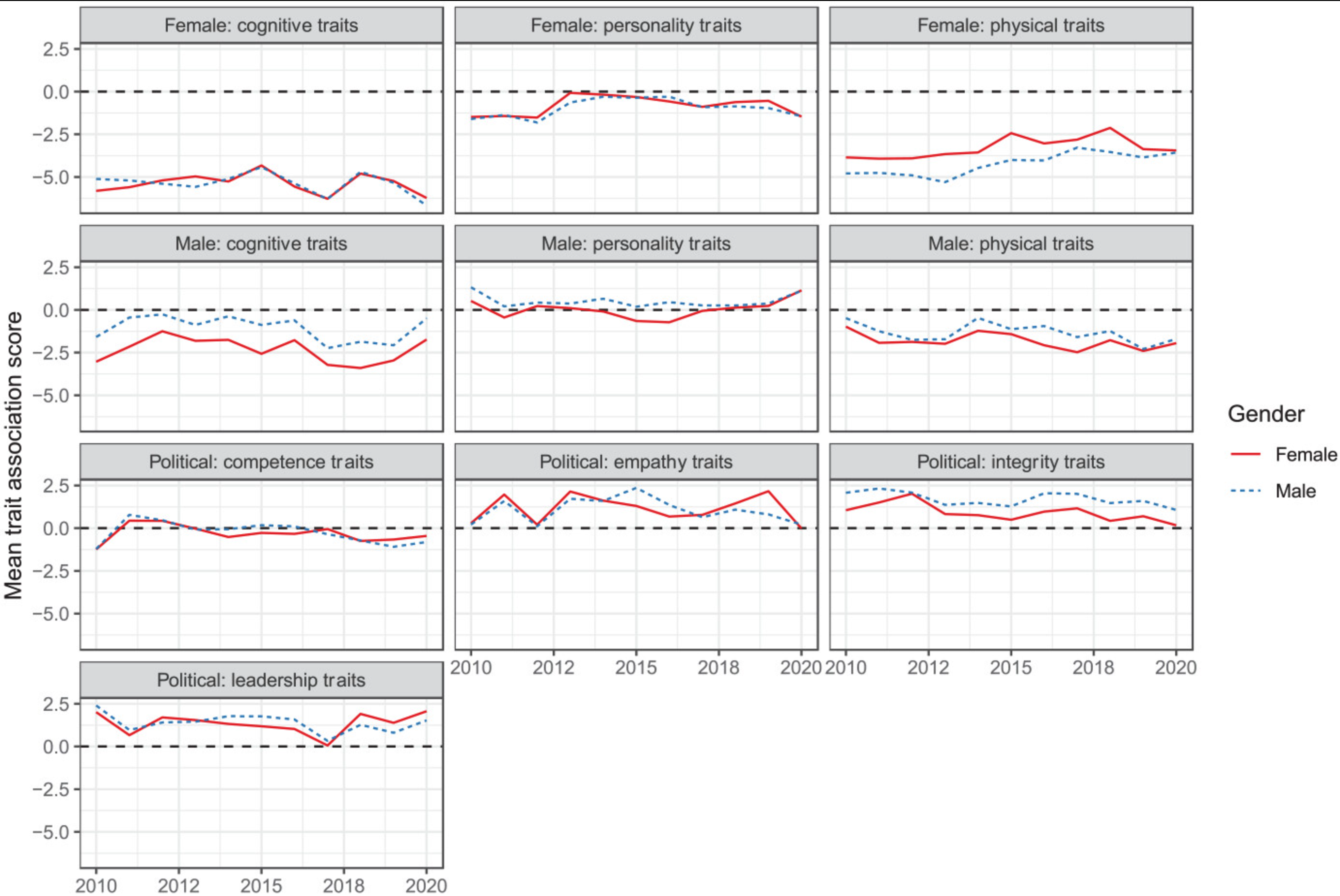
 Andrich et al. (2023) examine stereotypical traits in portrayals of 1,095 U.S. politicians.
Analyzed 5 million U.S. news stories published from 2010 to 2020 to study gender-linked (feminine, masculine) and political (leadership, competence, integrity, empathy) traits
Methodologically, they estimated word embeddings using the Continuous Bag of Words (CBOW) model, meaning that a target word (e.g., honest) is predicted from its context (e.g., Who thinks President Trump is [target word]?)
Bias can thus be identified if e.g., gender-neutral words (e.g., competent) are closer to words that represent one gender (e.g., donald_trump) than to words that represent the opposite gender (e.g., hillary_clinton).
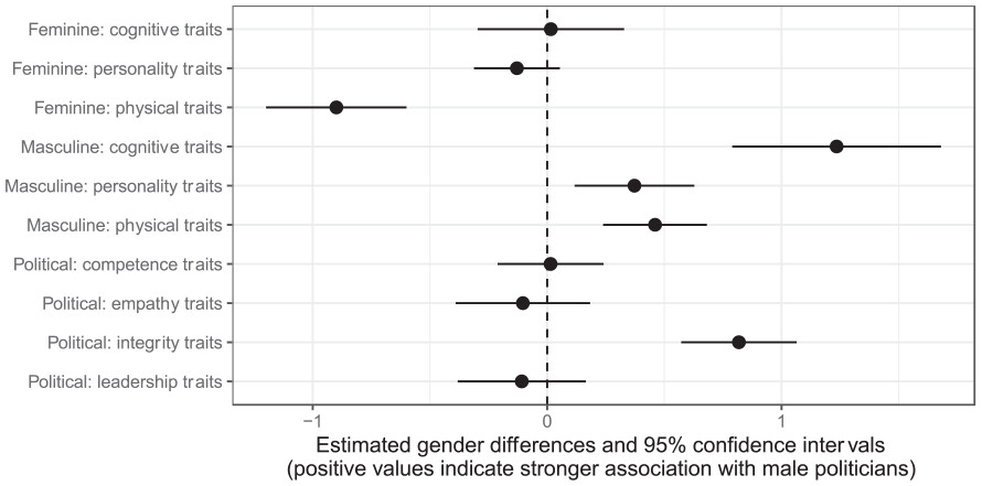
All three masculine traits were more strongly associated with male politicians.
In contrast, only the feminine physical traits were more strongly associated with female politicians.
Differences remained stable across time.
Improving Prediction by Using Word-Embeddings as Input Features
Word, sentence, or text embedding vectors can then be used as features in further text analysis tasks
Think about the example we just investigated: The sentence embeddings did capture some difference between:
Approaches from the last lecture (classic machine learning) would have a hard time to detect the negation “not great”.
Yet, bear in mind: We do not actually know what the 100+ (often >300) dimensions actually mean (→ we cannot look under the hood later!)
To fit a neural network based on static word-embeddings (e.g., GloVe), we only need to adapt the recipe.
Here, we do not need to engage in much preprocessing at all:
# Load GloVe embeddings (50-dimensional)
wv_tibble <- readr::read_delim("slides/GloVe 6B/glove.6B.300d.txt",
                               skip=1, delim=" ", quote="", col_names = c("word", paste0("d", 1:100)))

# Set up the recipe for text preprocessing with GloVe embeddings
text_rec <- recipe(label ~ text, data = science_data) |>
  step_tokenize(text) |>
  step_word_embeddings(text, embeddings = wv_tibble, aggregation = "mean") # <-- Here, I am adding the word-embeddings

# Define the MLP model specification
mlp_spec <-
  mlp(epochs = 400,          # <- times that algorithm will work through train set
      hidden_units = c(6),   # <- nodes in hidden units
      penalty = 0.01,        # <- regularization
      learn_rate = 0.2) |>   # <- shrinkage
  set_engine("brulee") |>    # <-- engine = R package
  set_mode("classification")

# Create workflow
mlp_wflow <- workflow()  |>
  add_recipe(text_rec) |>
  add_model(mlp_spec)

# Fit the workflow on the training data
mlp_fit <- mlp_wflow |>
fit(data = train_data)You may have noticed that I always set some hyperparameter in all of the models
There is no clear rule of how to set these parameters and their influence on performance is often unknown
We have to simply try out whether a neural network needs more than one hidden layer or how many nodes make sense, what learning rate works best, etc.
Good machine learning practice is to conduct a so-called grid-search, i.e. systematically run combinations of different specifications (but computationally expensive!!!)
Hvitfeld & Silge (2021)
# First, we update our model specification
mlp_spec <- mlp(hidden_units = tune(),   # <-- instead of fixed numbers, we set it to "tune"
                penalty = tune(),
                epochs = tune(),
                learn_rate = tune()) |>
  set_engine("brulee", trace = 0) |>
  set_mode("classification")
# Estract "dials" for parameter tuning
mlp_param <- extract_parameter_set_dials(mlp_spec)
# Simple combinatorial design
mlp_param |> grid_regular(levels = c(hidden_units = 2, penalty = 2, epochs = 2, learn_rate = 2)) # A tibble: 16 × 4
hidden_units penalty epochs learn_rate
<int> <dbl> <int> <dbl>
1 1 0.0000000001 5 0.001
2 10 0.0000000001 5 0.001
3 1 1 5 0.001
4 10 1 5 0.001
5 1 0.0000000001 500 0.001
6 10 0.0000000001 500 0.001
7 1 1 500 0.001
8 10 1 500 0.001
9 1 0.0000000001 5 0.316
10 10 0.0000000001 5 0.316
11 1 1 5 0.316
12 10 1 5 0.316
13 1 0.0000000001 500 0.316
14 10 0.0000000001 500 0.316
15 1 1 500 0.316
16 10 1 500 0.316# Combine the recipe and model into a workflow
mlp_wflow <- workflow() %>%
add_recipe(text_rec) %>%
add_model(mlp_spec)
# Set workflow with "dials"
mlp_param <- mlp_wflow |>
extract_parameter_set_dials() |>
update(epochs = epochs(c(100, 400)),
hidden_units = hidden_units(c(12, 64)),
penalty = penalty(c(-10, -1)),
learn_rate = learn_rate(range = c(-10, -1), trans = transform_log10()))
# Set metric of interest
acc <- metric_set(accuracy)
# Define resampling strategy
twofold <- vfold_cv(train_data, v = 2)
# Run the tuning process
mlp_reg_tune <- mlp_wflow |>
tune_grid(
resamples = twofold,
grid = mlp_param |>
grid_regular(levels = c(hidden_units = 2, penalty = 2, # <-- here, we set specific combination of parameters
epochs = 2, learn_rate = 2)), # instead, we could also use the `grid_random()`function
metrics = acc
)The result of this tuning grid search is a table that shows the best combinations of parameters in descending order
We can see here that 64 nodes, a very low penalty, a learning rate of 0.1 provides the best performance.
best_fit <- show_best(mlp_reg_tune, n = 48) |>
  select(-.estimator, -.config, -.metric) |>
  rename(accuracy = mean)
best_fit
# A tibble: 16 × 7
hidden_units penalty epochs learn_rate accuracy n std_err
<int> <dbl> <int> <dbl> <dbl> <int> <dbl>
1 64 0.0000000001 400 0.1 0.856 2 0.00406
2 64 0.0000000001 100 0.1 0.856 2 0.000980
3 12 0.0000000001 100 0.1 0.854 2 0.00406
4 64 0.1 400 0.1 0.784 2 0.00245
5 12 0.1 100 0.1 0.783 2 0.00287
6 12 0.1 400 0.1 0.782 2 0.00357
7 64 0.1 100 0.1 0.781 2 0.00371
8 12 0.0000000001 400 0.1 0.563 2 0.295
9 64 0.0000000001 400 0.0000000001 0.542 2 0.00154
10 64 0.1 400 0.0000000001 0.435 2 0.106
11 12 0.0000000001 100 0.0000000001 0.376 2 0.0277
12 64 0.0000000001 100 0.0000000001 0.328 2 0.216
13 12 0.0000000001 400 0.0000000001 0.327 2 0.216
14 12 0.1 400 0.0000000001 0.230 2 0.119
15 12 0.1 100 0.0000000001 0.228 2 0.120
16 64 0.1 100 0.0000000001 0.110 2 0.00126 mlp_best <-
mlp(epochs = 400, # <- times that algorithm will work through train set
hidden_units = c(64), # <- nodes in hidden units
penalty = 0.001, # <- regularization
learn_rate = 0.1) |> # <- shrinkage
set_engine("brulee") |> # <-- engine = R package
set_mode("classification")
# Create workflow
mlp_wflow_best <- workflow() |>
add_recipe(text_rec) |>
add_model(mlp_best)
# Fit the workflow on the training data
mlp_fit_best <- mlp_wflow_best |>
fit(data = train_data)Task difficulty
Amount of training data
Choice of features (n-grams, lemmata, etc)
Text preprocessing (e.g., exclude or include stopwords?)
Representation of text (tf, tf-idf, word-embedding)
Tuning of algorithm (what we just did in the grid search)
Scharkow ran a simple simulation study in which he systematically varied text preprocessing
The classifier was always Naive Bayes, below we see the average difference in performance
Van Atteveldt et al. (2021) re-analysised data reported in Boukes et al. (2020) to understand the validity of different text classification approaches for sentiment analysis
The data included news from a total of ten newspapers and five websites published between February 1 and July 7, 2015:
How Machine Learning is used in Communication Science
Su et al. (2018) examined the extent and patterns of incivility in the comment sections of 42 US news outlets’ Facebook pages in 2015–2016
News source outlets included
Implemented a combination of manual coding and supervised machine learning to code:
de León et al. (2021) explored how elections transform news sharing behaviour on Facebook
They investigated changes in news coverage and news sharing behaviour on Facebook
Employed a novel data set of news articles (N = 83,054) in Mexico
First coded 2,000 articles manually into topics (Politics, Crime and Disasters, Culture and Entertainment, Economic and Business, Sports, and Other), then used support vector machines to classify the rest

During periods of heightened political activity, both the publication and dissemination of political news increases
The gap between the news choices of journalists and consumers narrows, and increased political news sharing leading to a decrease in the sharing of other news.
Next week, we reach the present!
Machine learning in the social sciences generally used to solve an engineering problem
Output of Machine Learning is input for “actual” statistical model (e.g., we classify text, but run an analysis of variance with the output)
Ethical concerns
Is it okay to use a model we can’t possibly understand (e.g., SVM, neural networks)?
If they lead to false positives or false negatives, which in turn discriminate someone or lead to bias, it is difficult to find the source and denote responsibility
We always need to validate model on unseen and representative test data!
Think before you run models or you will waste a lot of computational resources
Classic machine learning is a useful tool for generalizing from a sample
It is very useful to reduce the amount of manual coding needed
Word-Embeddings are a dense representation of text that can improve speed and performance of standard ML approaches
That said, the field has moved on and innovations are fast-paced these days:

van Atteveldt, W., van der Velden, M. A. C. G., & Boukes, M.. (2021). The Validity of Sentiment Analysis: Comparing Manual Annotation, Crowd-Coding, Dictionary Approaches, and Machine Learning Algorithms. Communication Methods and Measures, (15)2, 121-140, https://doi.org/10.1080/19312458.2020.1869198
Su, L. Y.-F., Xenos, M. A., Rose, K. M., Wirz, C., Scheufele, D. A., & Brossard, D. (2018). Uncivil and personal? Comparing patterns of incivility in comments on the Facebook pages of news outlets. New Media & Society, 20(10), 3678–3699. https://doi.org/10.1177/1461444818757205
(available on Canvas)
Boumans, J. W., & Trilling, D. (2016). Taking stock of the toolkit: An overview of relevant automated content analysis approaches and techniques for digital journalism scholars. Digital journalism, 4(1), 8-23.
de León, E., Vermeer, S. & Trilling, D. (2023). Electoral news sharing: a study of changes in news coverage and Facebook sharing behaviour during the 2018 Mexican elections. Information, Communication & Society, 26(6), 1193-1209. https://doi.org/10.1080/1369118X.2021.1994629
Hvitfeld, E. & Silge, J. (2021). Supervised Machine Learning for Text Analysis in R. CRC Press. https://smltar.com/
Lantz, B. (2013). Machine learning in R. Packt Publishing Ltd.
Scharkow, M. (2013). Thematic content analysis using supervised machine learning: An empirical evaluation using german online news. Quality & Quantity, 47(2), 761–773. https://doi.org/10.1007/s11135-011-9545-7
Su, L. Y.-F., Xenos, M. A., Rose, K. M., Wirz, C., Scheufele, D. A., & Brossard, D. (2018). Uncivil and personal? Comparing patterns of incivility in comments on the Facebook pages of news outlets. New Media & Society, 20(10), 3678–3699. https://doi.org/10.1177/1461444818757205
van Atteveldt, W., van der Velden, M. A. C. G., & Boukes, M.. (2021). The Validity of Sentiment Analysis: Comparing Manual Annotation, Crowd-Coding, Dictionary Approaches, and Machine Learning Algorithms. Communication Methods and Measures, (15)2, 121-140, https://doi.org/10.1080/19312458.2020.1869198
Van Atteveldt and colleagues (2020) tested the validity of various automated text analysis approaches. What was their main result?
A. English dictionaries performed better than Dutch dictionaries in classifying the sentiment of Dutch news paper headlines.
B. Dictionary approaches were as good as machine learning approaches in classifying the sentiment of Dutch news paper headlines.
C. Of all automated approaches, supervised machine learning approaches performed the best in classifying the sentiment of Dutch news paper headlines.
D. Manual coding and supervised machine learning approaches performed similarly well in classifying the sentiment of Dutch news paper headlines.
How are word embeddings learned?
A. By assigning random numerical values to each word
B. By analyzing the pronunciation of words
C. By scanning the context of each word in a large corpus of documents
D. By counting the frequency of words in a given text
How are word embeddings learned?
A. By assigning random numerical values to each word
B. By analyzing the pronunciation of words
C. By scanning the context of each word in a large corpus of documents
D. By counting the frequency of words in a given text
Describe the typical process used in supervised text classification.
Any supervised machine learning procedure to analyze text usually contains at least 4 steps:
One has to manually code a small set of documents for whatever variable(s) you care about (e.g., topics, sentiment, source,…).
One has to train a machine learning model on the hand-coded /gold-standard data, using the variable as the outcome of interest and the text features of the documents as the predictors.
One has to evaluate the effectiveness of the machine learning model via cross-validation. This means one has to test the model test on new (held-out) data.
Once one has trained a model with sufficient predictive accuracy, precision and recall, one can apply the model to more documents that have never been hand-coded or use it for the purpose it was designed for (e.g., a spam filter detection software)

Computational Analysis of Digital Communication