 Model relation between…

 Simple model cannot combine features


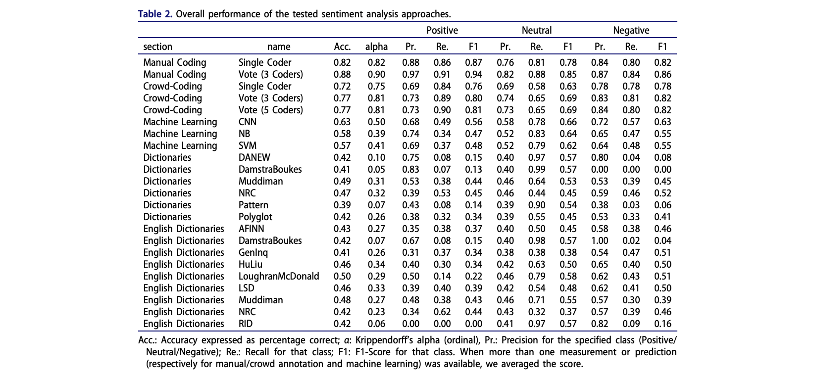
Main results
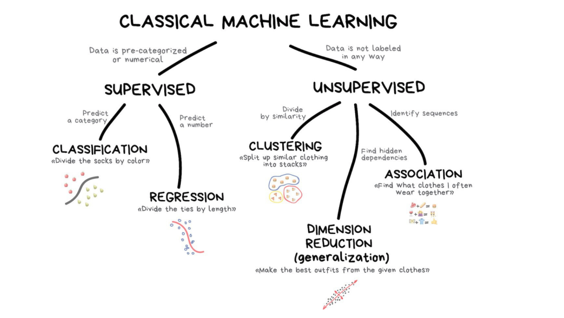
Week 3: Supervised Text Classification
Having no more need for human programmers, humankind is simply deleted…
Is this what machine learning is about?
(Stills from the movies “Ex Machina” and “Her”)


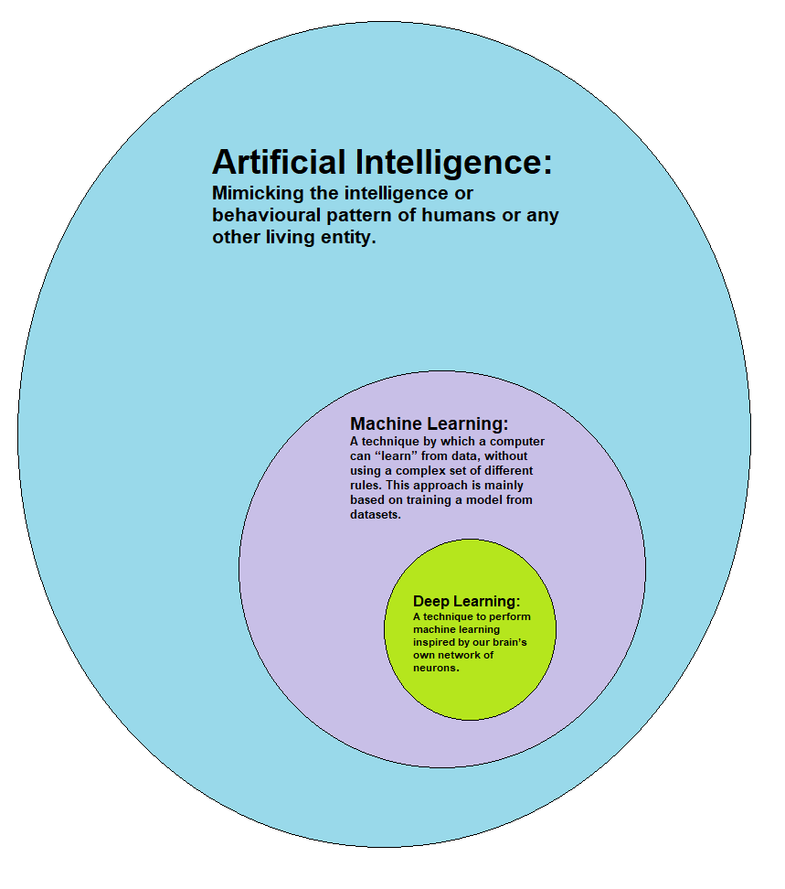 Machine learning is most successful when it augments, rather than replaces, the specialized knowledge of a subject-matter expert.
Machine learning is used in a wide variety of applications and contexts, such as in businesses, hospitals, scientific laboratories, or governmental organizations
In communication science, we can use these techniques to automate text analysis!
Lantz, 2013
 Applying machine learning in practical context:
Machine learning is thus similar to normal statistical modeling
Learn \(f\) so you can predict \(y\) from \(x\):
y based on x.
 Computes the prior probability ( P ) for every category ( c = outcome variable ) based on the training data set
Computes the probability of every feature ( x ) to be a characteristic of the class ( c ); i.e., the relative frequency of the feature in category
For every probability of a category in light of certain features ( P(c|X) ), all feature probabilities ( x ) are multiplied
The algorithm hence chooses the class that has highest weighted sum of inputs
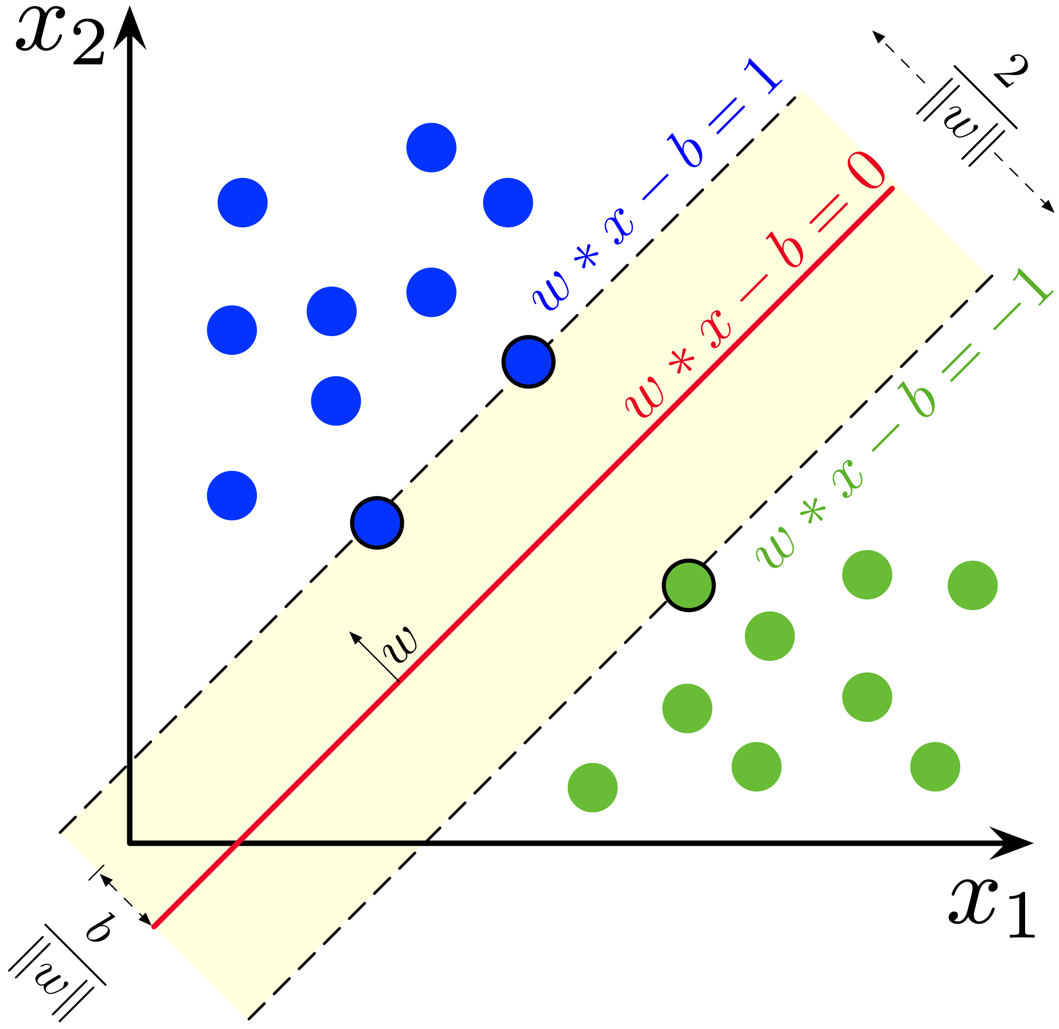 Very often used machine learning method
Can be imagined as a “surface” that creates a boundary between points of data plotted in a multidimensional space representing examples and their feature values
Tries to find decision boundary between points that maximizes margin between classes while minimizing errors
More formally, a support-vector machine constructs a hyperplane or set of hyperplanes in a high- or infinite-dimensional space
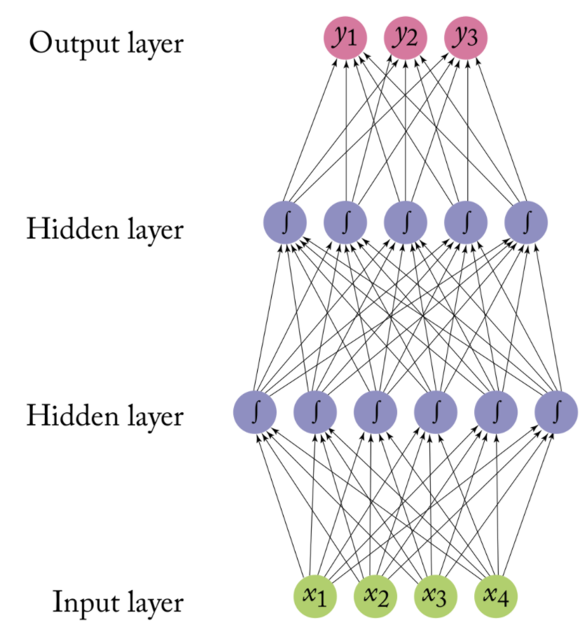
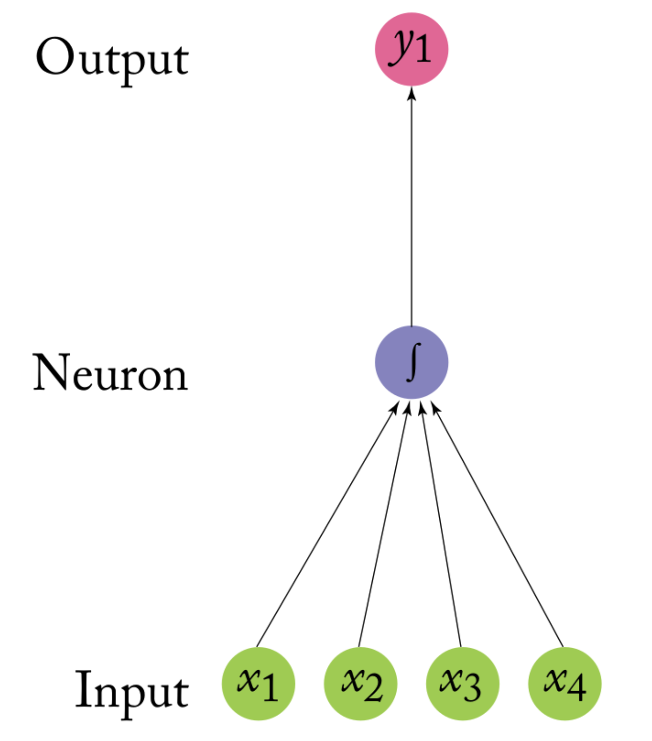 Inspired by human brain (but abstracted to mathematical model)
Each ‘neuron’ is a linear model with activation function:
\(y = f(w_1x_1 + … + w_nx_n)\)
Normal activation functions: logistic, linear, block, tanh, …
Each neuron is practically a generalized linear model
Networks differ with regard to three main characteristics:
Contains artist name, song name, lyrics, and genre of the artist (not the song)
The following genres are in the data set:
bind_rows(cm_nb2, cm_svm2) %>%
  bind_cols(Model = c(rep("Naive Bayes", 3),
                      rep("SVM", 3))) %>%
  pivot_longer(Precision:F1) %>%
  ggplot(aes(x = Genre,
             y = value,
             fill = Model)) +
  geom_bar(stat= "identity",
           position = "dodge",
           color = "white") +
  scale_fill_brewer(palette = "Pastel1") +
  facet_wrap(~name) +
  coord_flip() +
  ylim(0, 1) +
  theme_grey() +
  theme(legend.position = "bottom")
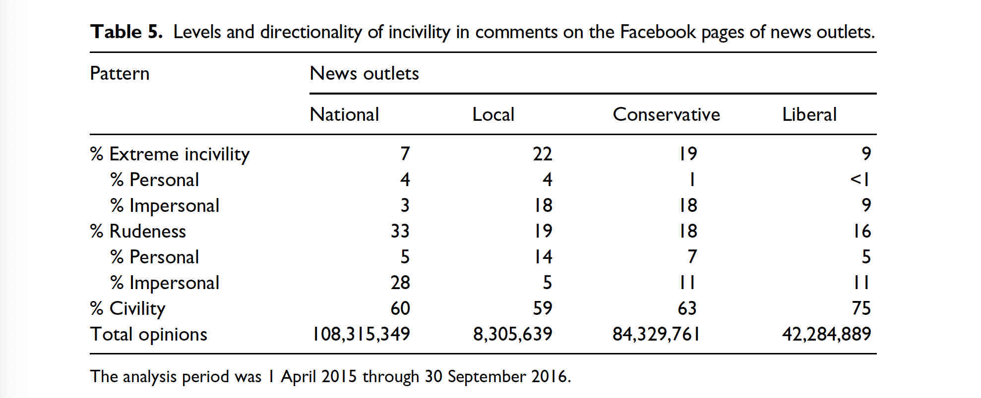
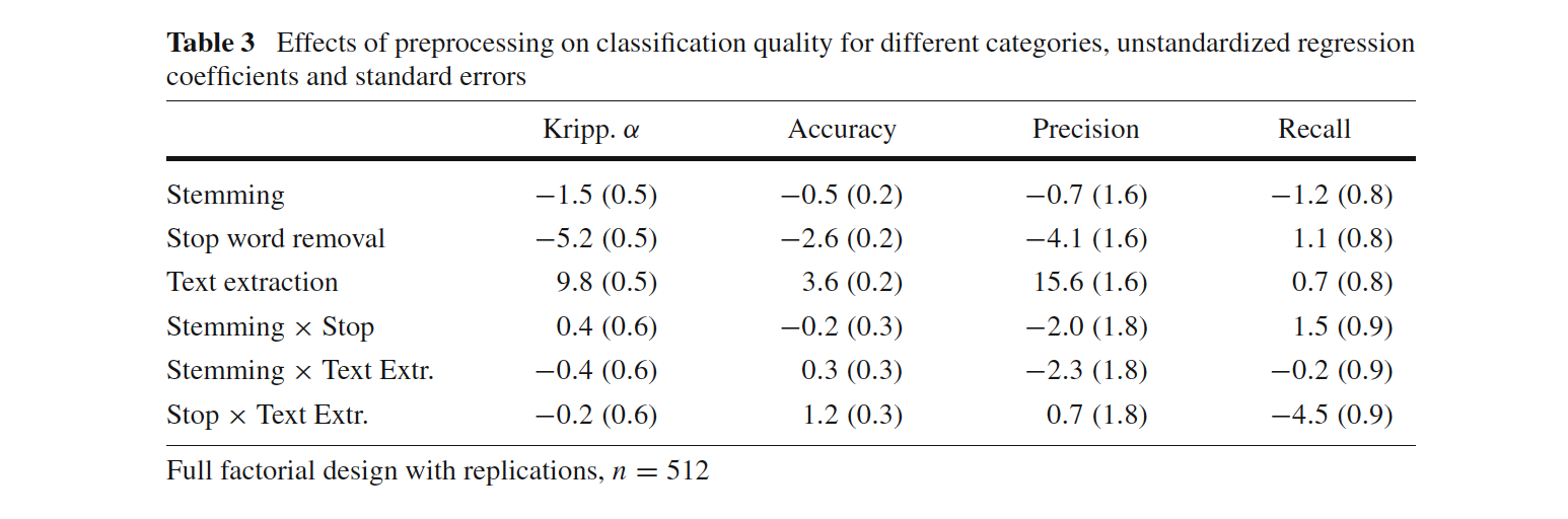
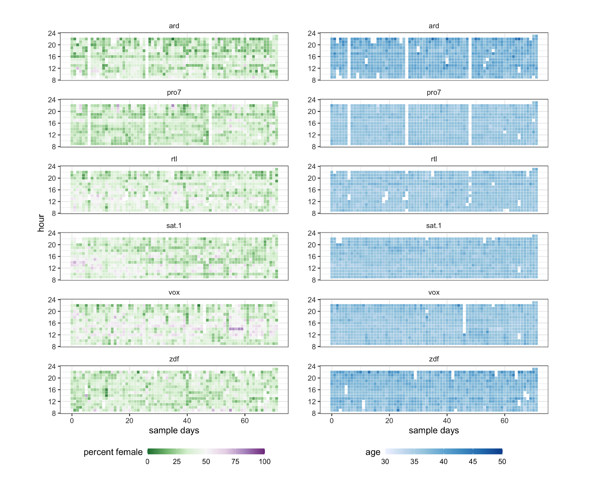
Scharkow, 2013
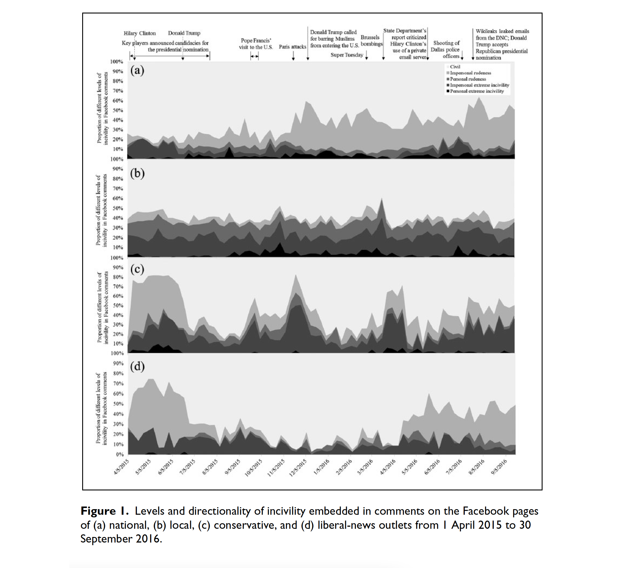
Despite several discernible spikes, the percentage of extremely uncivil personal comments on national-news outlets’ pages shifted only modestly
On conservative outlets’ Facebook pages, the proportions of both extremely uncivil and rude comments fluctuated dramatically across the sampling window
Su et al., 2018
There is a new package (very recently released) that allows to use such pre-trained, large scale language models in R
If you are interested check the package “text”: https://r-text.org/
But: Be mindful! Running a BERT model can take a long time and might even require a more powerful computer than yours!
![]()
Machine learning is a useful tool for generalizing from sample
It is very useful to reduce the amount of manual coding needed
Many different models exist (each with many parameters/options)
We always need to validate model on unseen and representative test data!
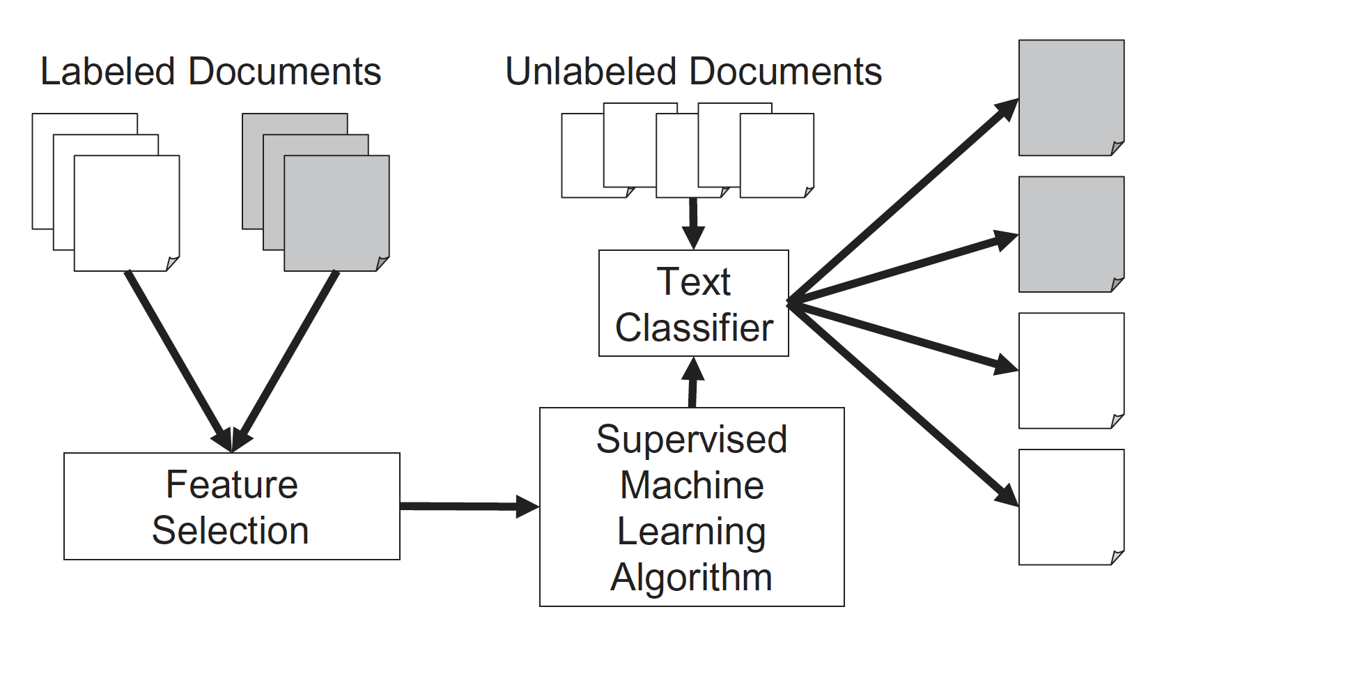
Describe the typical process used in supervised text classification.
Any supervised machine learning procedure to analyze text usually contains at least 4 steps:
One has to manually code a small set of documents for whatever variable(s) you care about (e.g., topics, sentiment, source,…).
One has to train a machine learning model on the hand-coded /gold-standard data, using the variable as the outcome of interest and the text features of the documents as the predictors.
One has to evaluate the effectiveness of the machine learning model via cross-validation. This means one has to test the model test on new (held-out) data.
Once one has trained a model with sufficient predictive accuracy, precision and recall, one can apply the model to more documents that have never been hand-coded or use it for the purpose it was designed for (e.g., a spam filter detection software)
![]()