# Load data
library(tidyverse)
url <- "https://raw.githubusercontent.com/vanatteveldt/ecosent/master/data/intermediate/sentences_ml.csv"
d <- read_csv(url) |>
  select(id, text = headline, lemmata, sentiment=value) |>
  mutate(sentiment = factor(sentiment, levels = c(-1, 0, 1),
                            labels = c("negative", "neutral", "positive")))
head(d)Word Embeddings, Transformers, and Large Language Models
Week 4: Bert, GPT, and Co
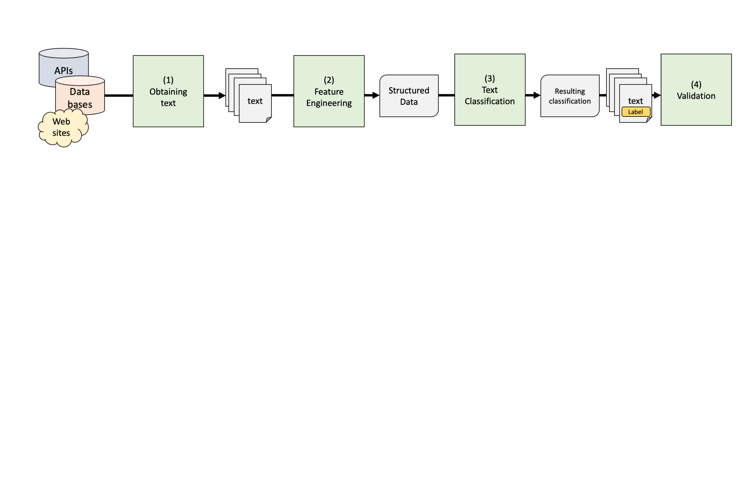
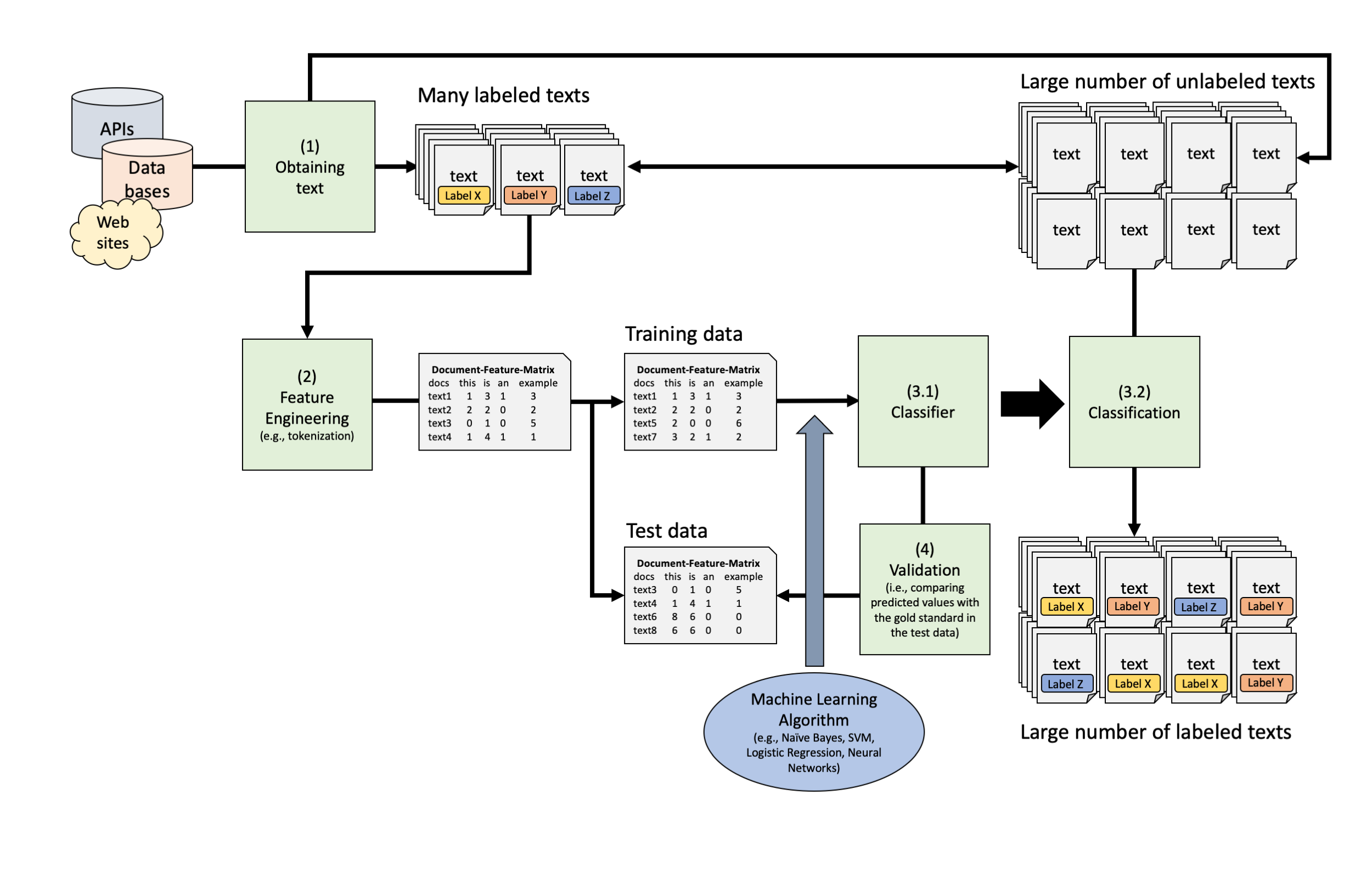
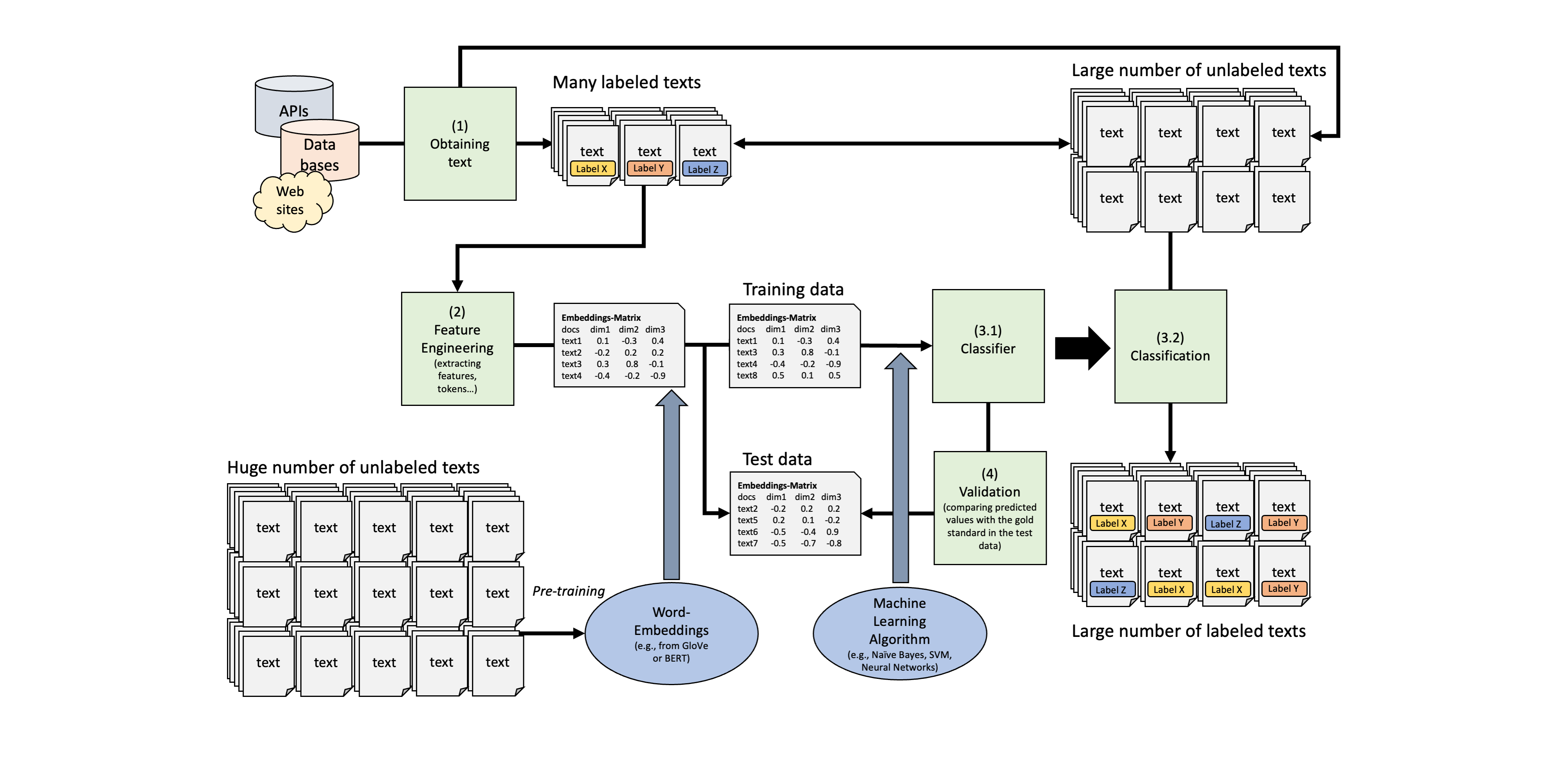
Text Classification Pipeline
Machine Learning (1990-2010)
And now?
Rember: The initial problem of text analysis
Computers don’t read text, they only can deal with numbers
For this reason, so far, we tokenized our texts (e.g., in words) and summarized their frequency across texts to create a document-feature matrix within the bag-of-words model
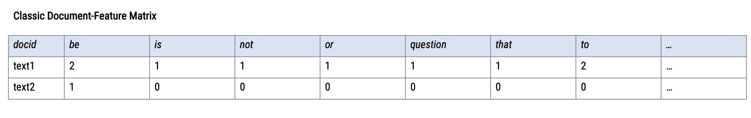
Such a text representation has some issues:
- Treats words as equally important (→ requires removal of noise, stopwords…)
- Ignores word order and context
- Results in a sparse matrix (→ computationally expensive)
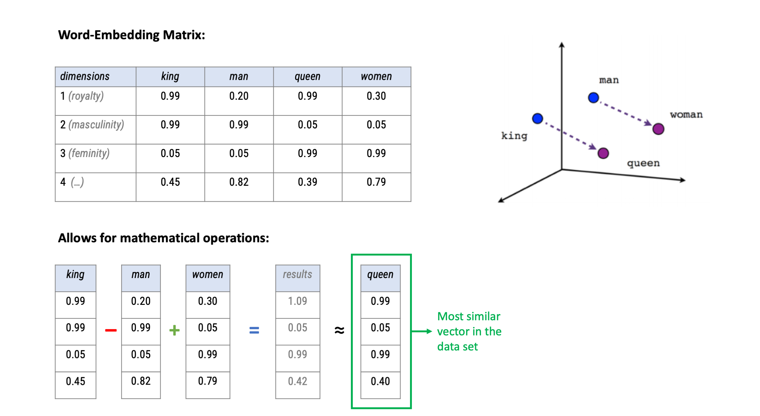
Alternative: Map words into a vector space
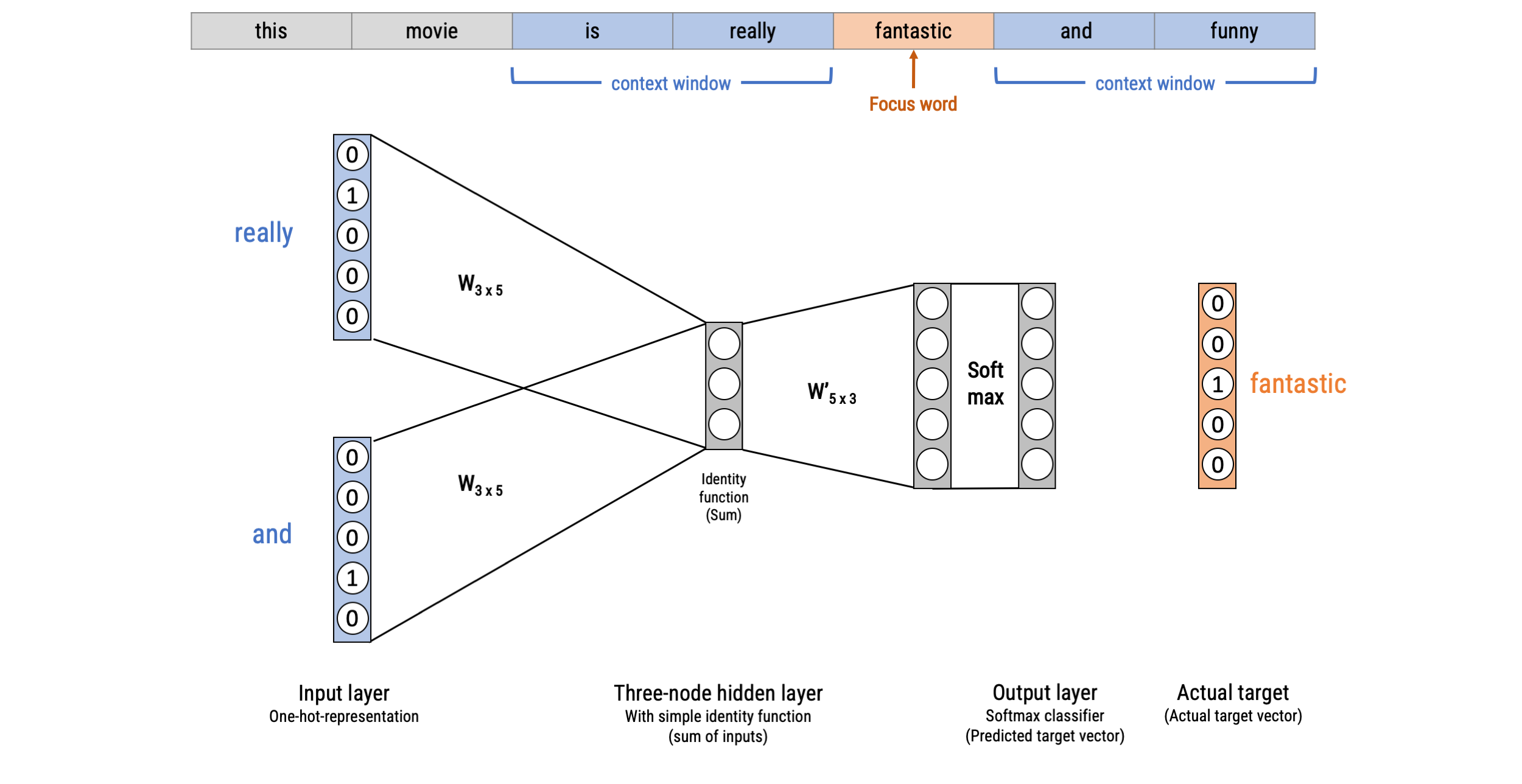
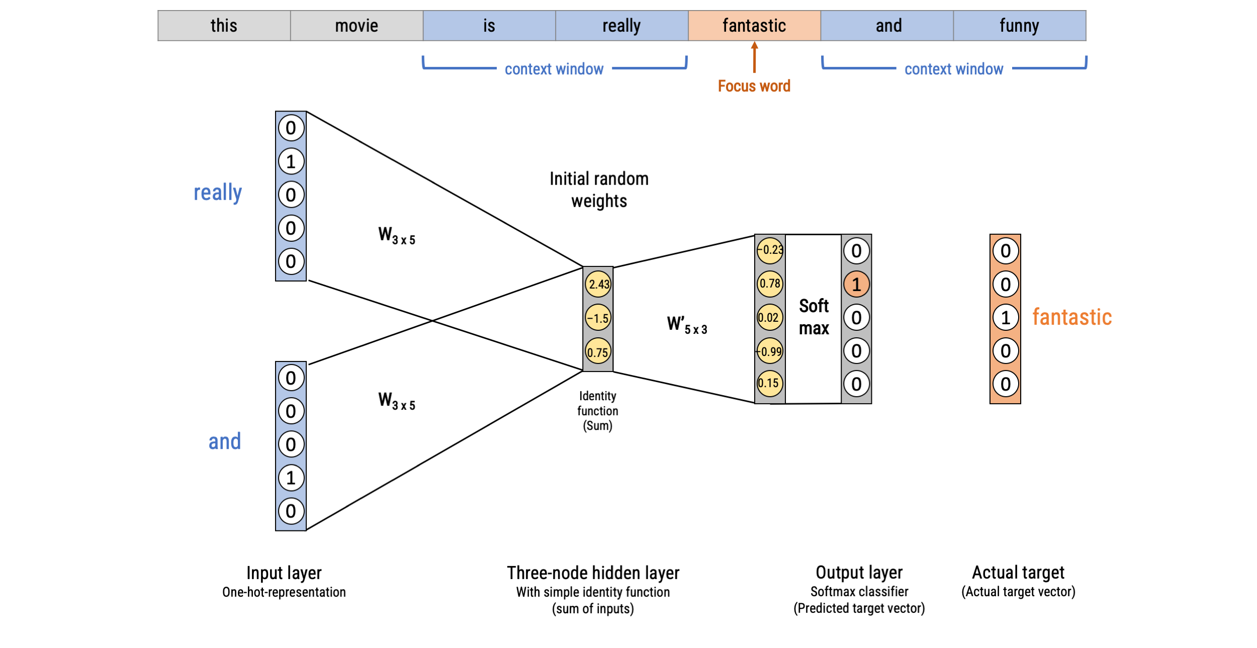
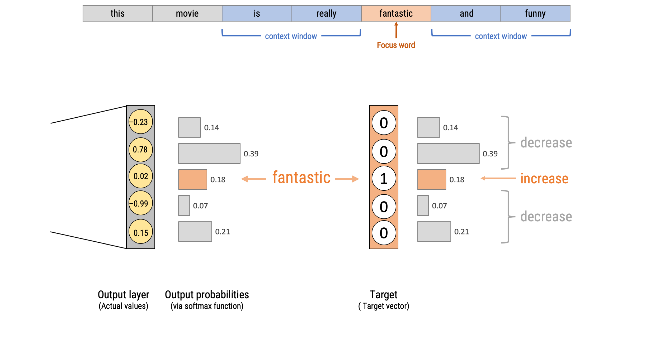
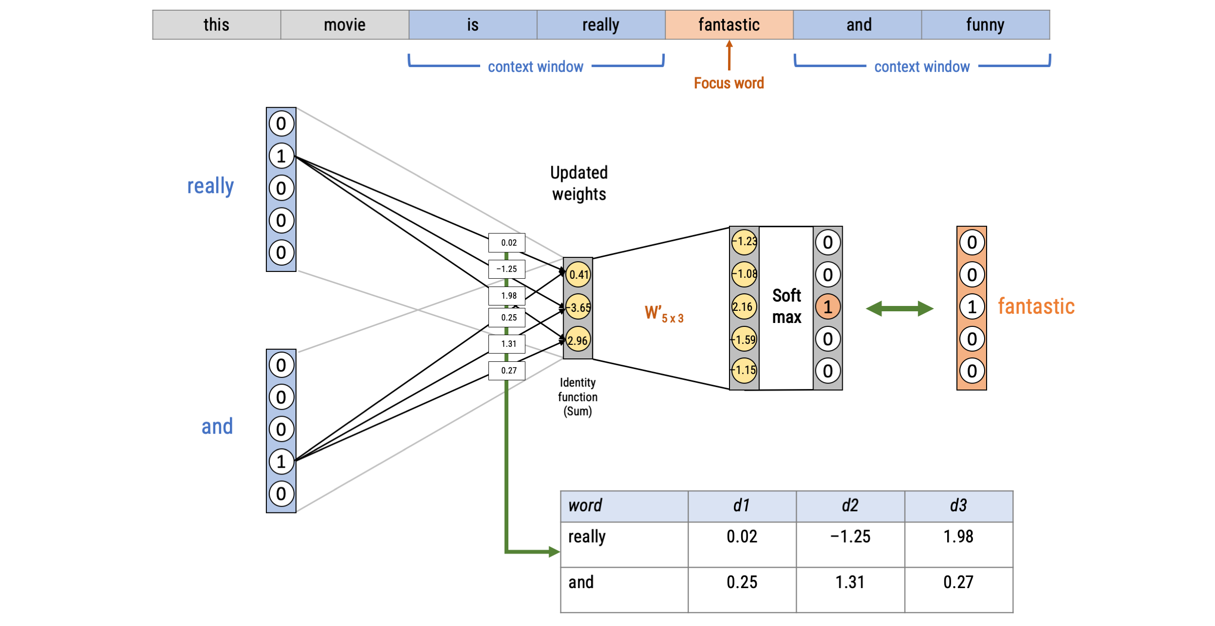
Word2Vec: Continuous Bag-of-words (CBOW)
Word2Vec: Continuous Bag-of-words (CBOW)
Word2Vec: Continuous Bag-of-words (CBOW)
Word2Vec: Continuous Bag-of-words (CBOW)
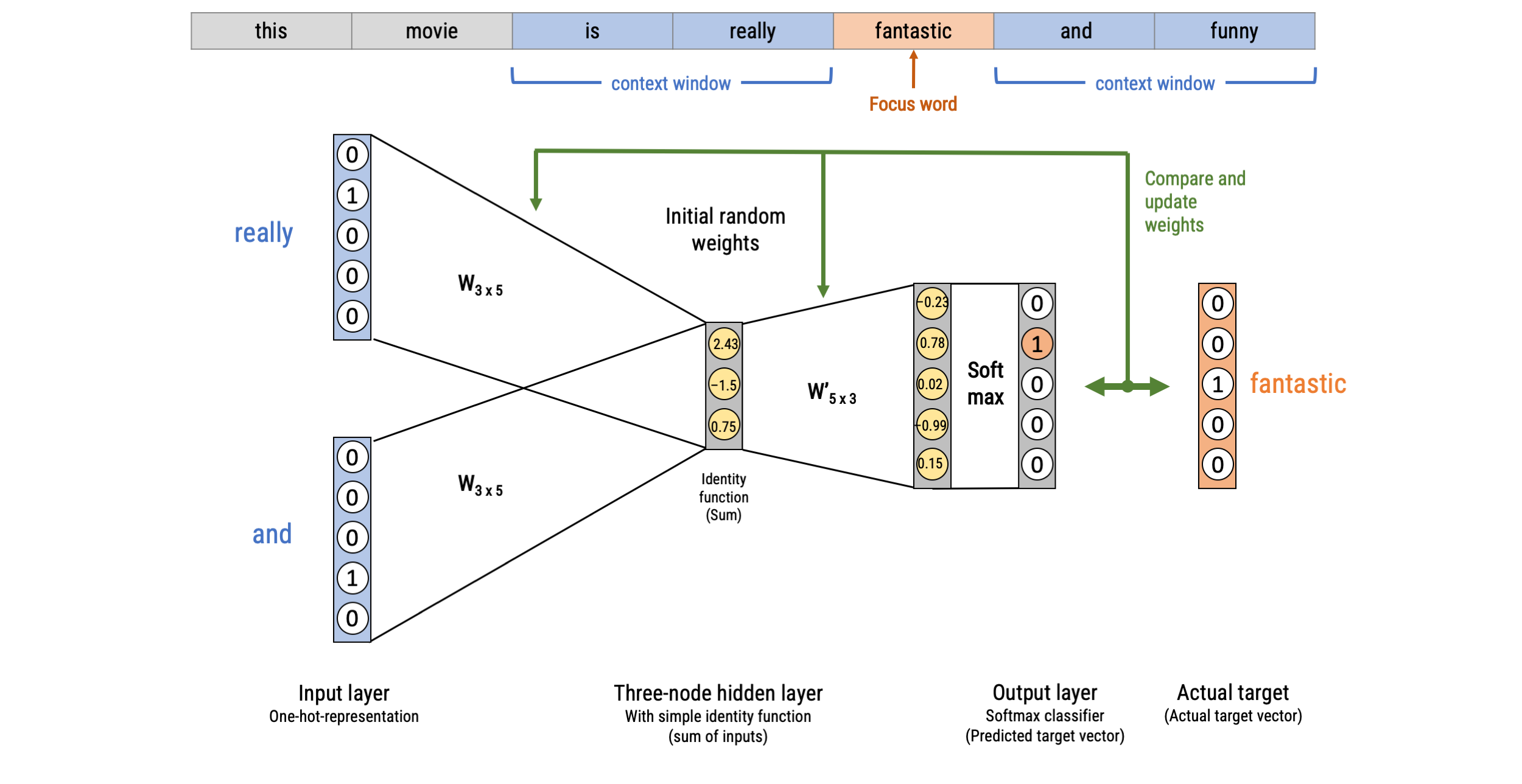
Word2Vec: Continuous Bag-of-words (CBOW)
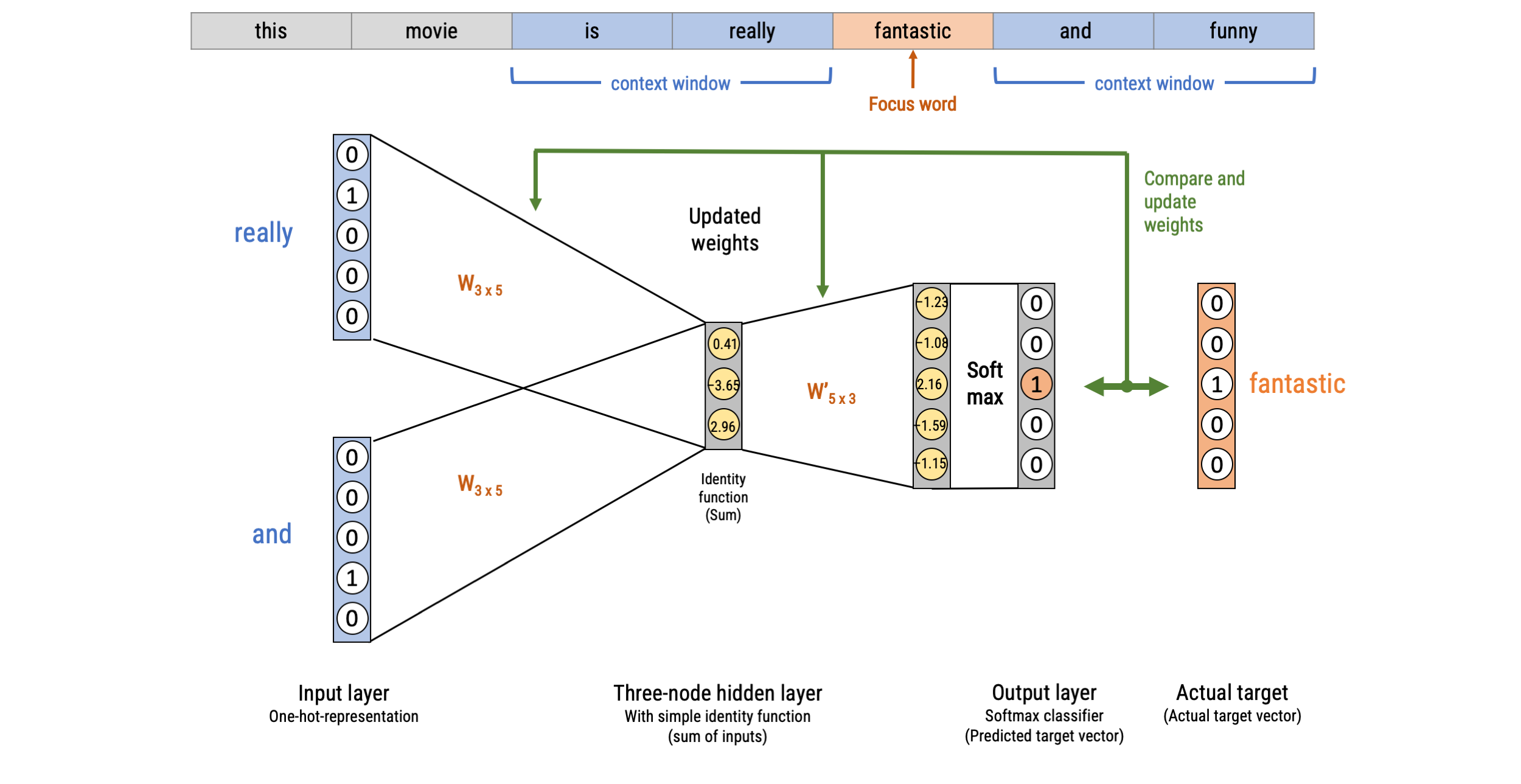
Word2Vec: Continuous Bag-of-words (CBOW)
Text classification with Word-Embeddings
Doing analysis with word-embedding themselves
Based on vector-based computations, we can also analyse semantic relationships
This is a quite common approach by now in research on gender and other types of stereotypes
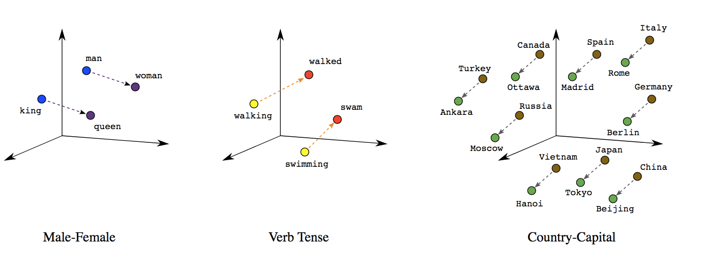
Source: https://developers.google.com
Example from the literature: Gender-Stereotypes
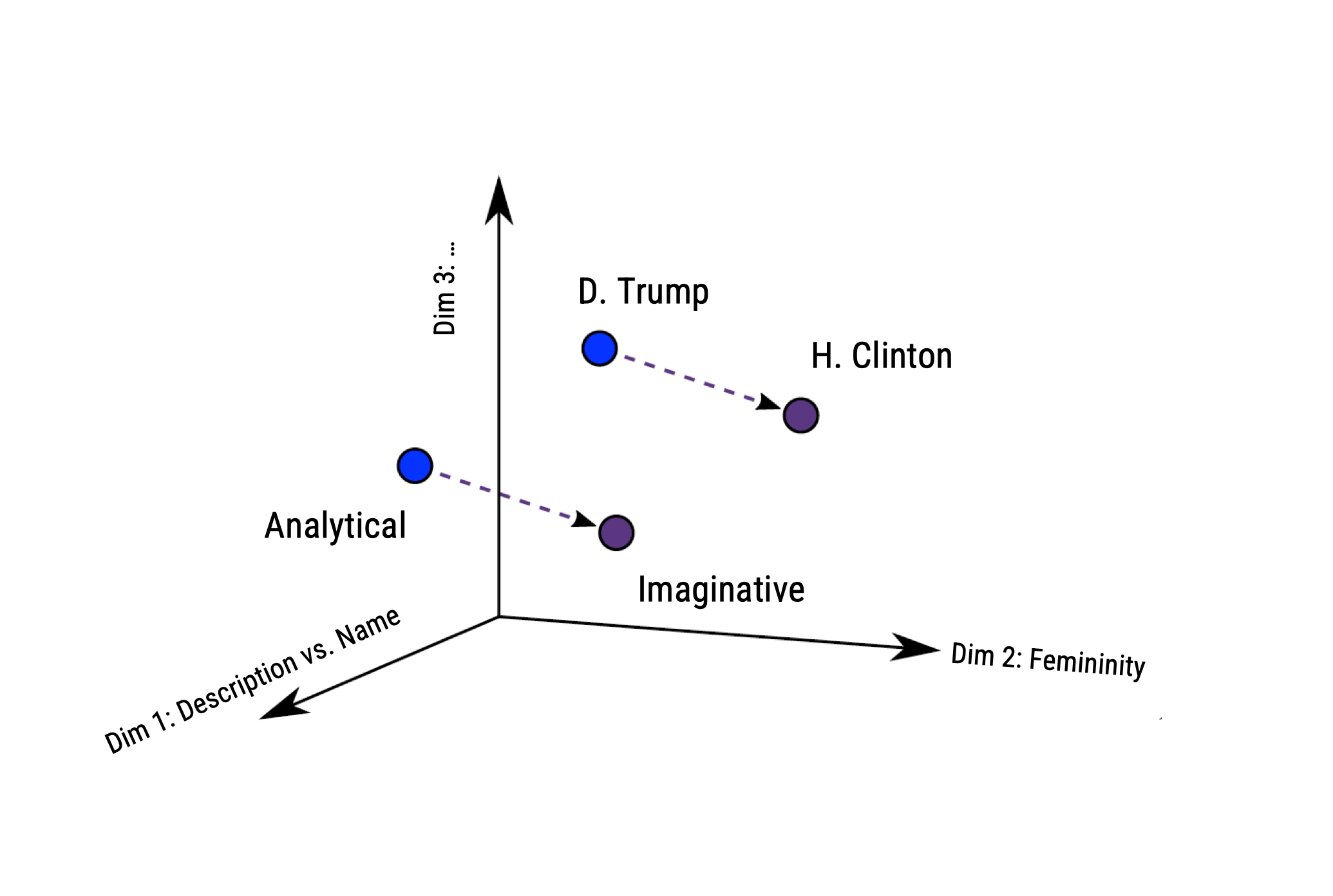
![]() Andrich et al. (2023) examine stereotypical traits in portrayals of 1,095 U.S. politicians.
Andrich et al. (2023) examine stereotypical traits in portrayals of 1,095 U.S. politicians.Analyzed 5 million U.S. news stories published from 2010 to 2020 to study gender-linked (feminine, masculine) and political (leadership, competence, integrity, empathy) traits
Methodologically, they estimated word embeddings using the Continuous Bag of Words (CBOW) model, meaning that a target word (e.g., honest) is predicted from its context (e.g., Who thinks President Trump is [target word]?)
Bias can thus be identified if e.g., gender-neutral words (e.g., competent) are closer to words that represent one gender (e.g., donald_trump) than to words that represent the opposite gender (e.g., hillary_clinton).
 Andrich et al. (2023) examine stereotypical traits in portrayals of 1,095 U.S. politicians.
Results
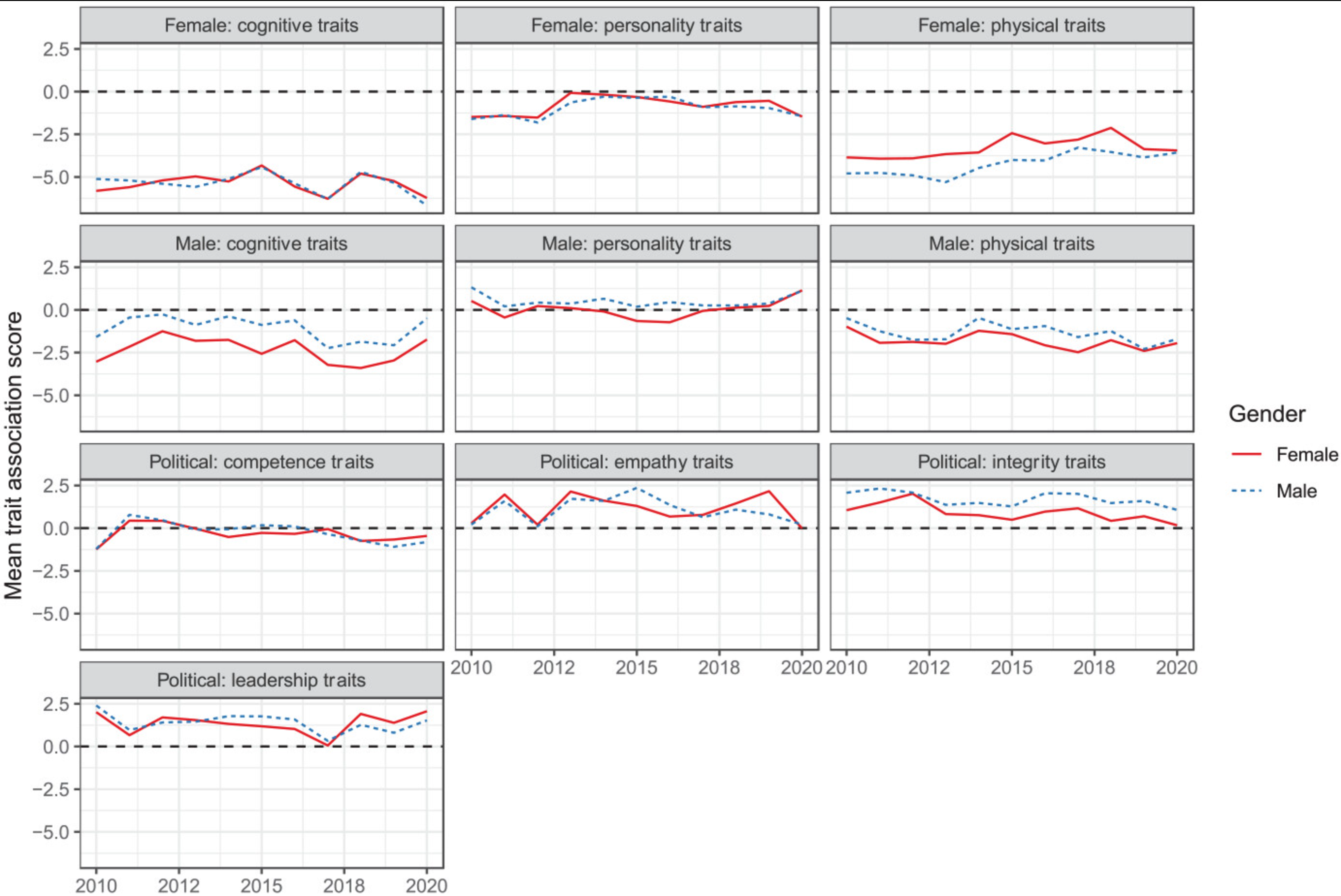
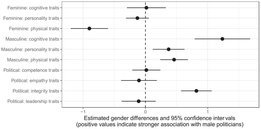
All three masculine traits were more strongly associated with male politicians.
In contrast, only the feminine physical traits were more strongly associated with female politicians.
Differences remained stable across time.
The Rise of Transformers and Transfer Learning
OVerview of the architecture
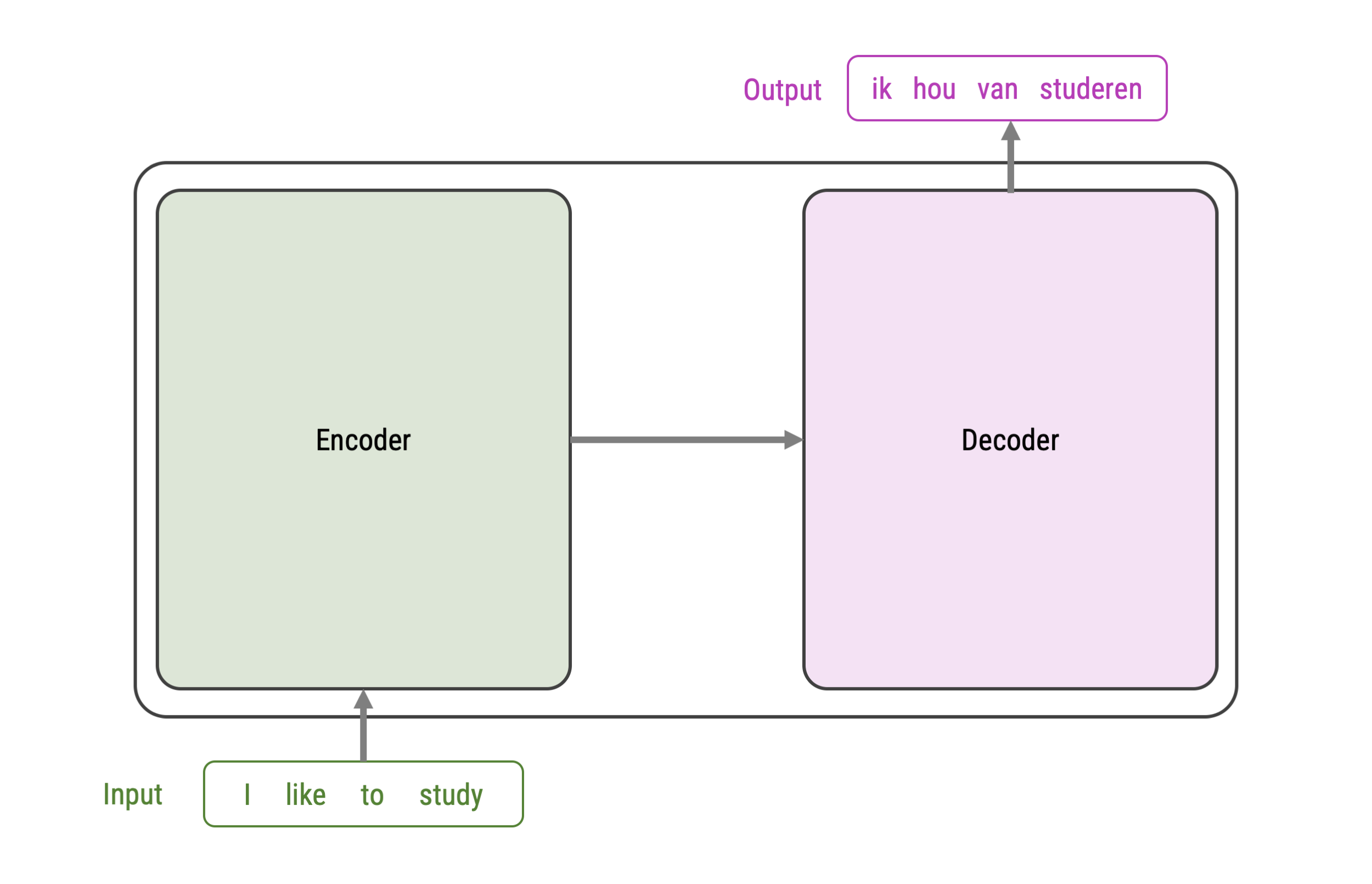
The figure on the right represent an abstract overview of a transformer’s architecture
It can be used for sequence-to-sequence predictions
- classic example is translation: e.g., english-to-dutch
- but also: question-to-answer, text-to-summary, sentence-to-next-sentence…
Although models can differ, they generally include:
- An encoder-decoder framework
- Word embeddings + positional embedding
- Attention and self-attention modules
We won’t cover any of these in much detail and just aim for a high-level understanding
Vaswani et al. 2017
![]()
Basic Encoder-Decoder Framework (for Translation)
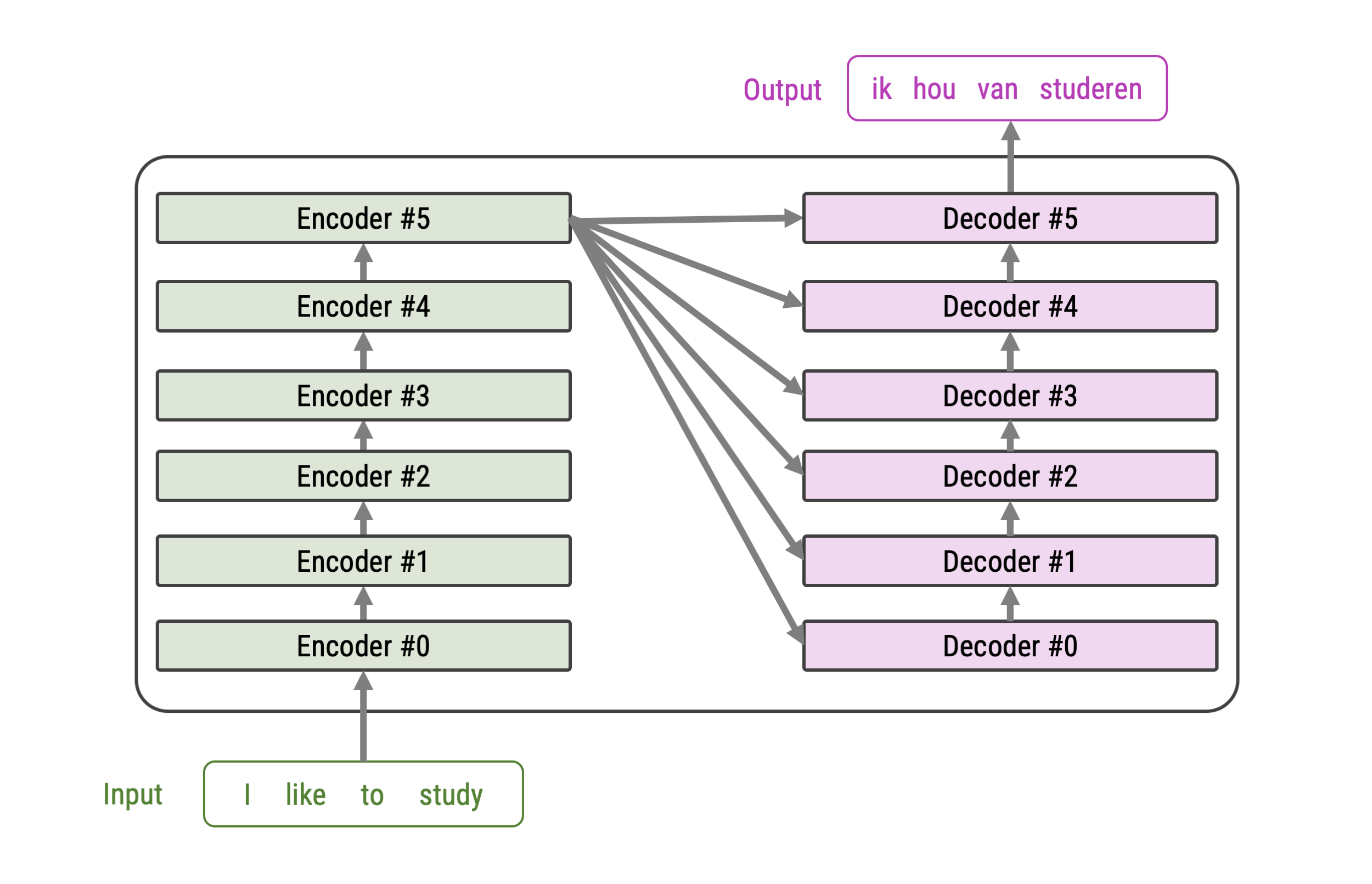
Stacked Encoders and Decoders
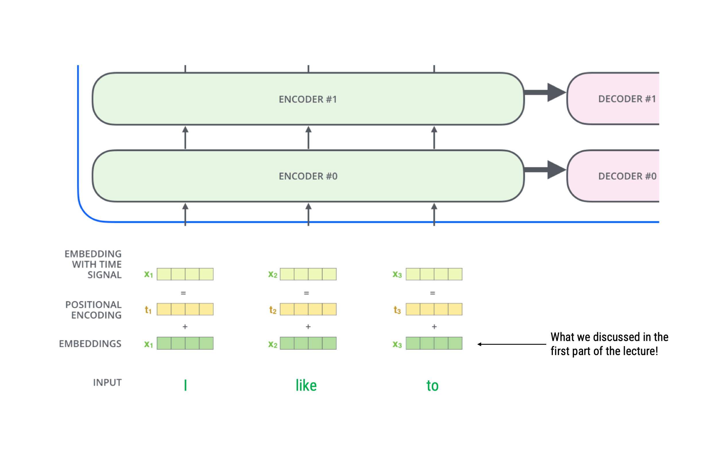
More elaborate encoding of words
Source: Alammar, 2018
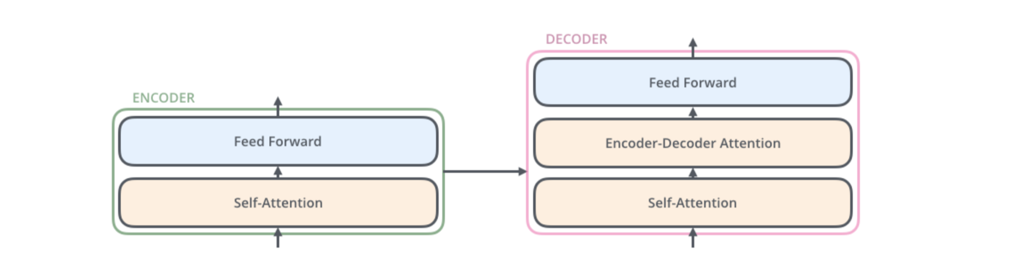
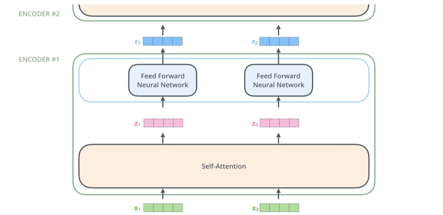
Inside of an encoder and a decoder
The word, position, and time signal embeddings are passed to the first encoder
Here, they flow through a self-attention layer, which further refines the encoding by “looking at other words” as it encodes a specific word
The outputs of the self-attention layer are fed to a feed-forward neural network.
The decoder likewise has both layers as well, but also an extra attention layer that helps to focus on different parts of the input (e.g., the encoders outputs)
Source: Alammar, 2018
Encoding pipeline
The embedding only happens in the bottom-most encoder.
In other encoders, it would be the output of the encoder that’s directly below.
Source: Alammar, 2018
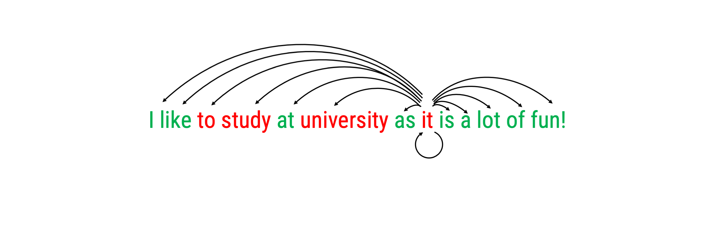
Self-Attention
In general terms, self-attention works encodes how similar each word is to all the words in the sentence, including itself.
Once the similarities are calculated, they are used to determine how the transformers encodes each word.

Self-Attention
In general terms, self-attention works encodes how similar each word is to all the words in the sentence, including itself.
Once the similarities are calculated, they are used to determine how the transformers encodes each word.

Self-Attention
In general terms, self-attention works encodes how similar each word is to all the words in the sentence, including itself.
Once the similarities are calculated, they are used to determine how the transformers encodes each word.

Self-Attention
In general terms, self-attention works encodes how similar each word is to all the words in the sentence, including itself.
Once the similarities are calculated, they are used to determine how the transformers encodes each word.
Putting it all together
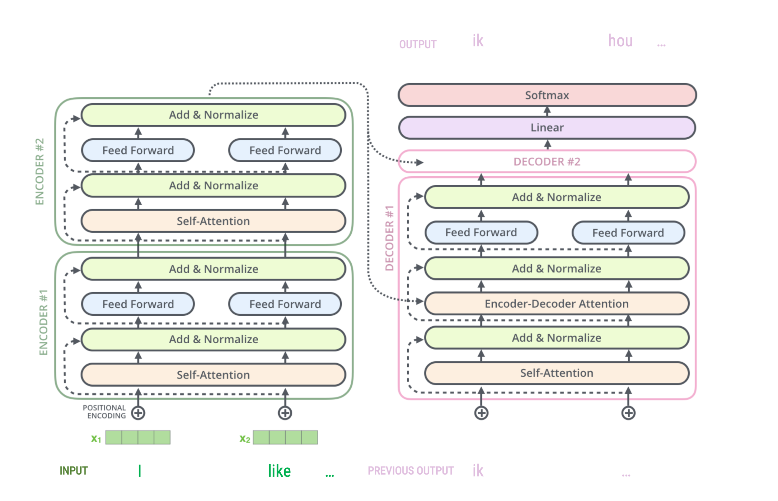
Source: Alammar, 2018
High-level process
The transformers starts by creating word embeddings (combinations of similarity, position, time signal)
The encoder start by processing the input sequence (embeddings).
The output of the top encoder is then transformed into a set of attention vectors which are used by each decoder in its “encoder-decoder attention” layer which helps the decoder focus on appropriate places in the input sequence
The decoder spits out a first output (e.g., the word “I”), which then becomes the input for the decoder in follow-up steps
The decoder repeats these steps until a special symbol (e.g.,
= “end of sentence”) is reached.
![]()
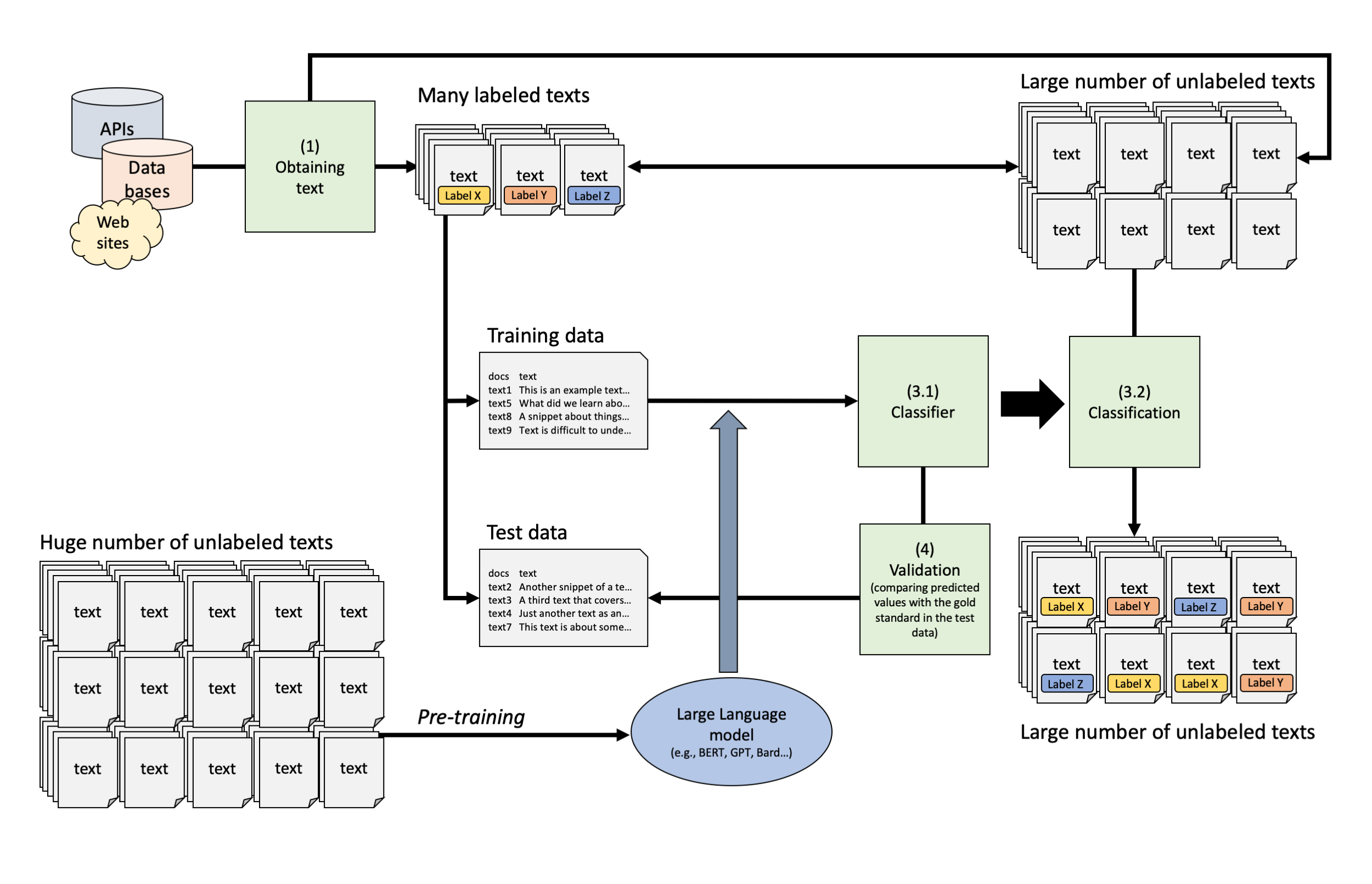
Text Classification Pipeline Using Transformers
Large Language Models: BERT, GPT and the “AI Revolution”?
Source: Christian Behler on Medium
Next token prediction (as in GPT-2)
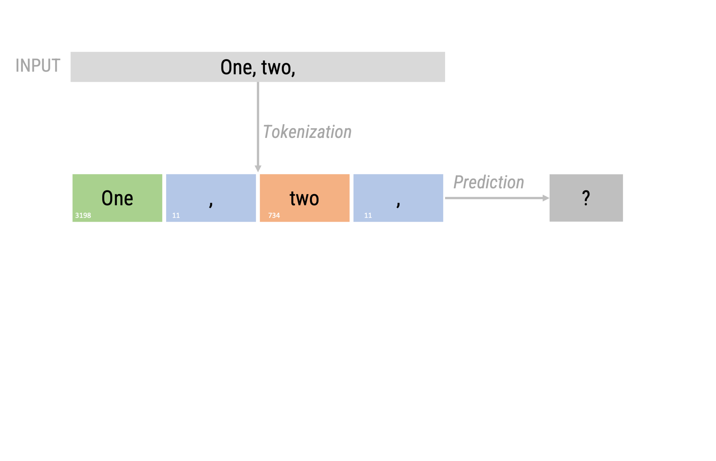
Next token prediction (as in GPT-2)
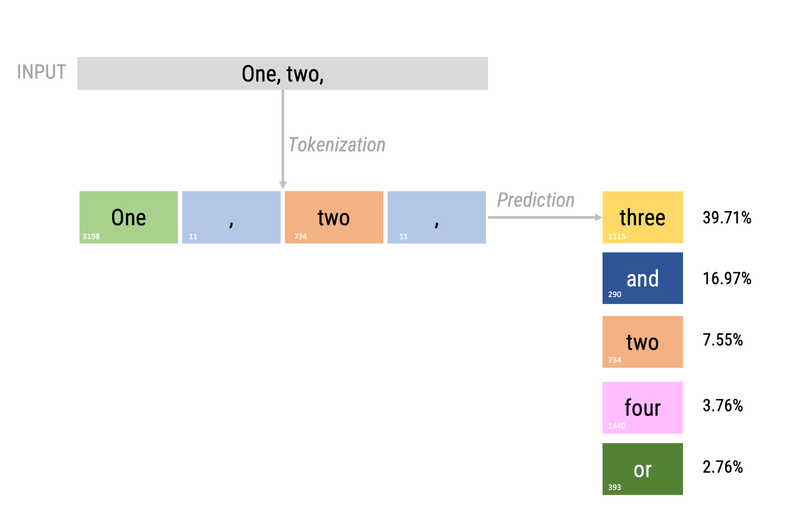
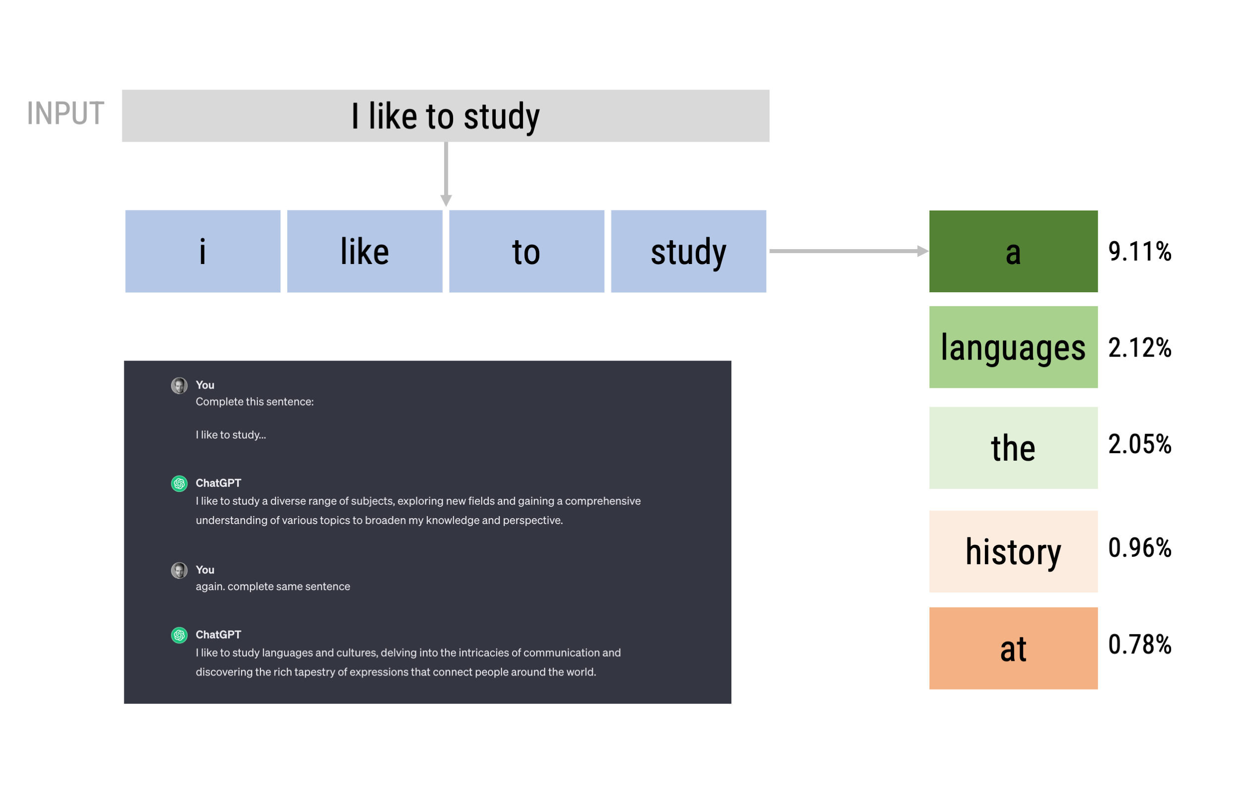
Next token prediction
Bert
Bidirectional Encoder Representations from Transformers (BERT) is a family of language models introduced in October 2018 by researchers at Google.
BERT is an “encoder-only” transformer architecture.
Generally speaking, BERT consists of three modules:
- Embedding. This module converts an array of one-hot encoded tokens into an array of vectors representing the tokens.
- Stack of encoders. These encoders are the Transformer encoders (BERT-base = 12, BERT-large = 24). They perform transformations over the array of representation vectors.
- Un-embedding. This module converts the final representation vectors into one-hot encoded tokens again.
Devlin et al. 2018

Training and Fine-Tuning of BERT
Pretrained on two task:
- Mask Language Modelling (LM): simply mask some percentage of the input tokens at random, and then predict those masked tokens
- Next sentence prediction (NSP): predict sentence B from sentence A to model relationships between sentences
This pre-training led to great performances in downstream tasks
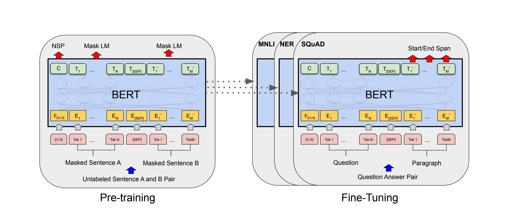
Source: Devlin et al., 2018
GPT-Series by OpenAI
Generative Pre-trained Transformer (GPT), is a set of state-of-the-art large language model developed by OpenAI.
Particularly GPT-3, released publicly in November 2022 together with a chat interface, caused a lot of public attention.
Millions of users in a very short amount of time (faster than Facebook, Instagram, TikTok, etc…), now 1.5 Billion users
![]()
High-level architecture and training of GPT
- GPT are decoder-only models
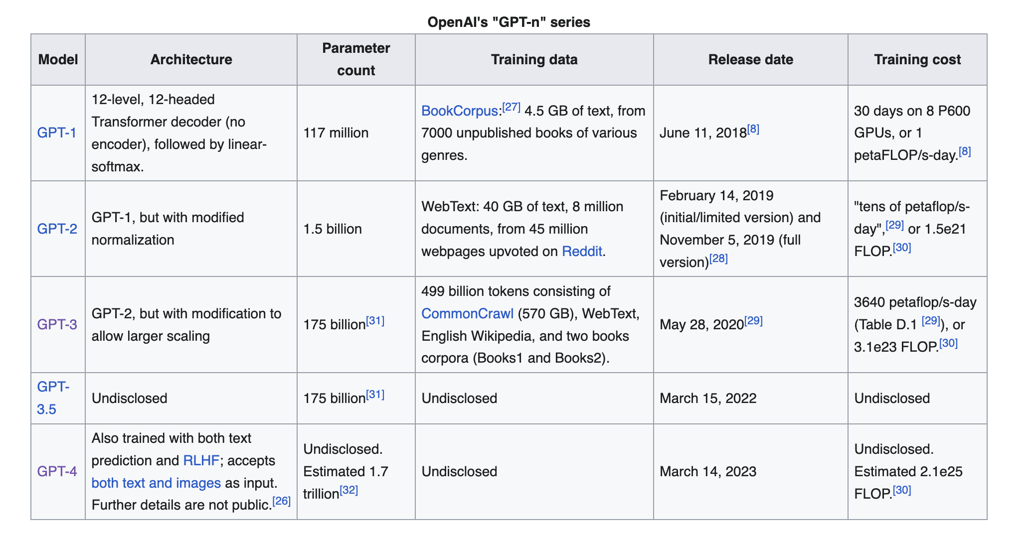
Source: Wikipedia
Zero-Shot Text Classification with LLMS
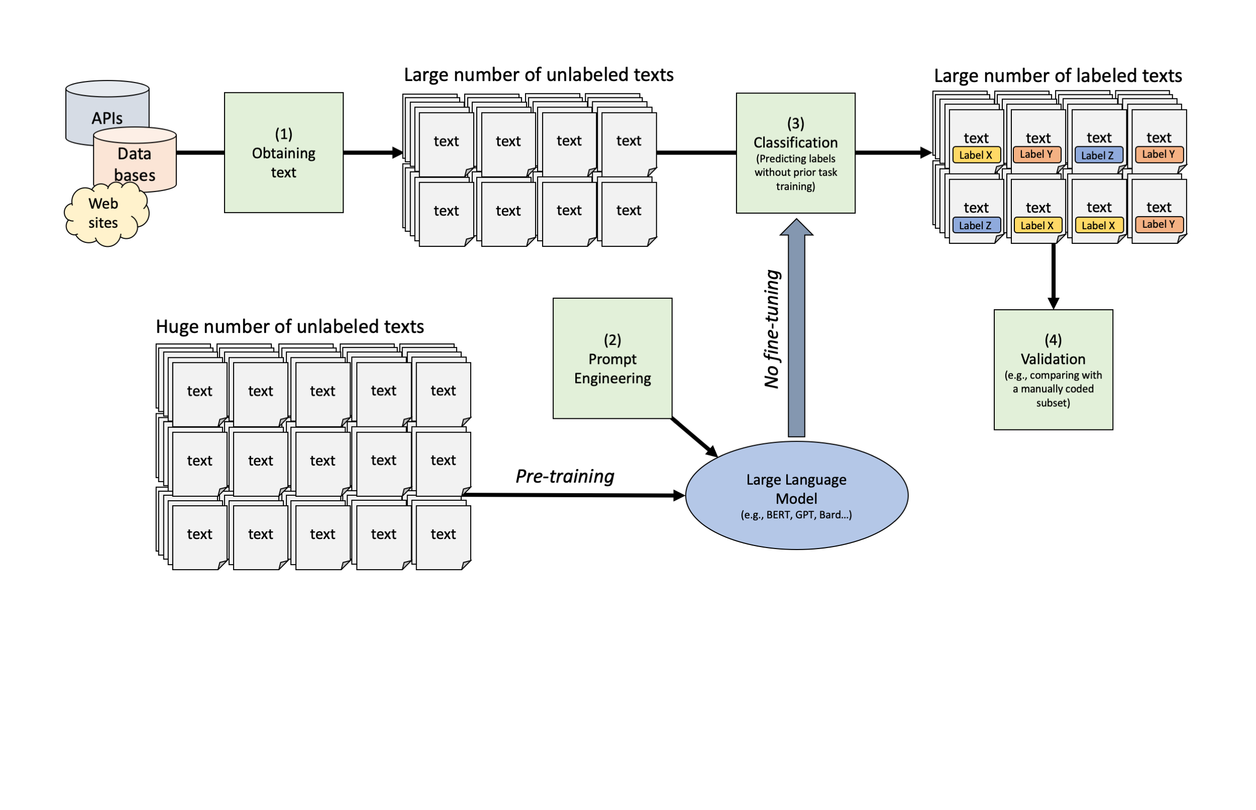
Many LLMS are available at huggingface.co

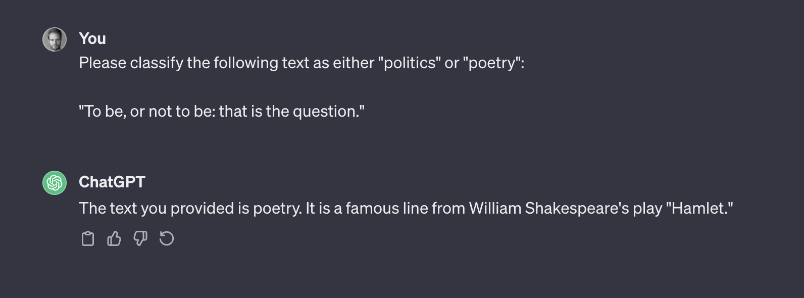
Using GPT for text classification
- The simplest way to use GPT is to simply paste text into the chat and ask for the relevant topics (in fact, let’s try this now!)
Yet, for larger text corpora this is not feasible
To use GPT for text analysis purposes, we need to access the models via the Open AI API
- We created functions that allow to use the GPT models similarly to how we used the hugging face models
- Requires to pay per token (luckily not too expensive, we will provide some accounts)
Comparison between neural network and GPT-3.5
We can see that the neural network does better overall, but bear in mind that it was trained on a lot of data (10,445 songs!)
GPT-3.5 yields a quite astonishing performance, given that it was not trained to do this task at all!
bind_rows(
  predict_ann |>
  class_metrics(truth = actual,
                estimate = predicted) |>
  mutate(approach = "classic ML: neural network"),
  predict_gpt |>
  class_metrics(truth = binary_genre,
                estimate = labels) |>
  mutate(approach = "zero-shot learning: gpt-3.5")
 ) |>
  ggplot(aes(x = .metric, y = .estimate,
             fill = approach)) +
  geom_col(position = position_dodge()) +
  geom_text(aes(y = .estimate -.05,
                label = round(.estimate, 2)),
            position = position_dodge(width = .75)) +
  ylim(0, 1) +
  coord_flip() +
  theme(legend.position = "bottom") +
  labs(x = "", y = "Score", fill = "")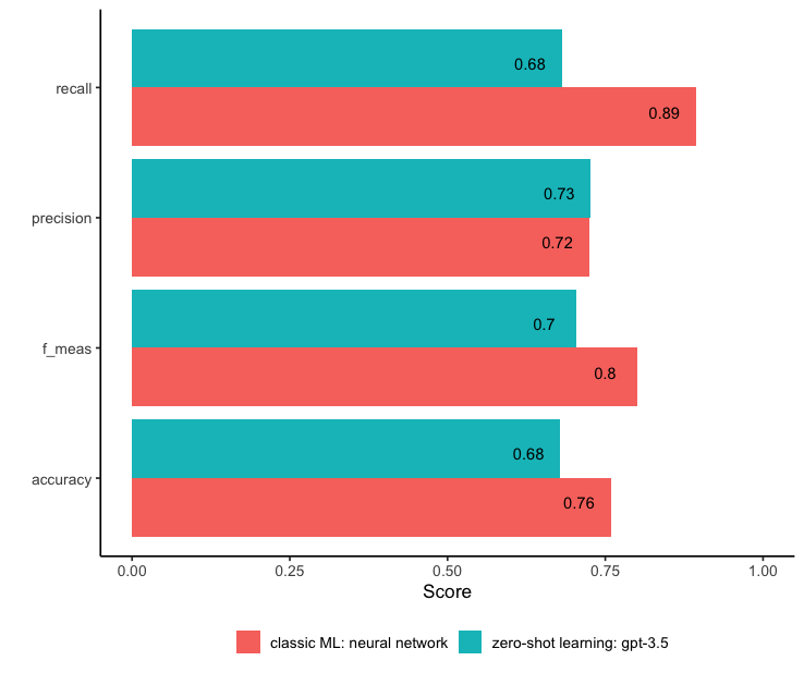
Examples in the literature
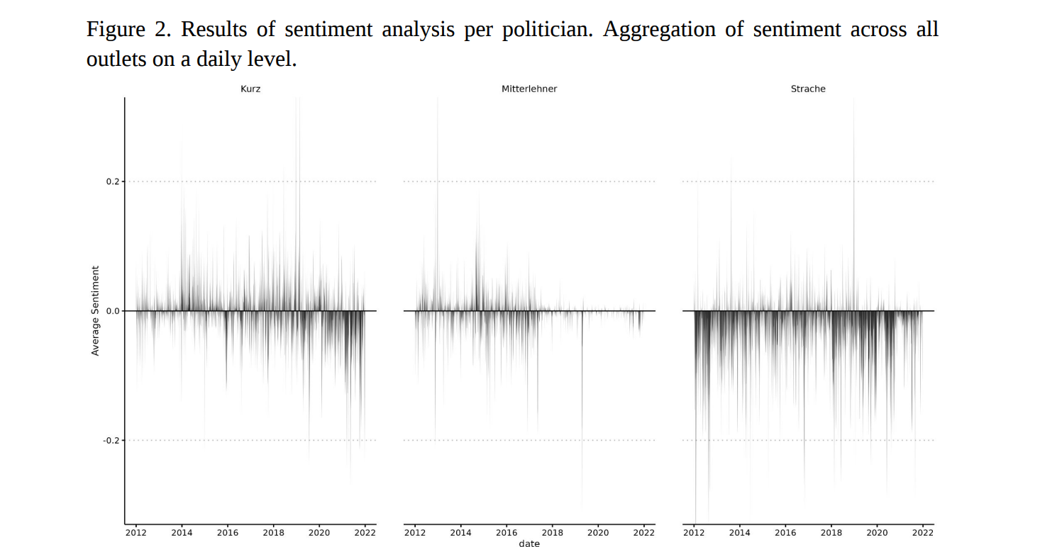
Baluff et al. (2023) investigated a recent case of media capture, a mutually corrupting relationship between political actors and media organizations.
This case involves former Austrian chancellor who allegedly colluded with a tabloid newspaper to receive better news coverage in exchange for increased ad placements by government institutions.
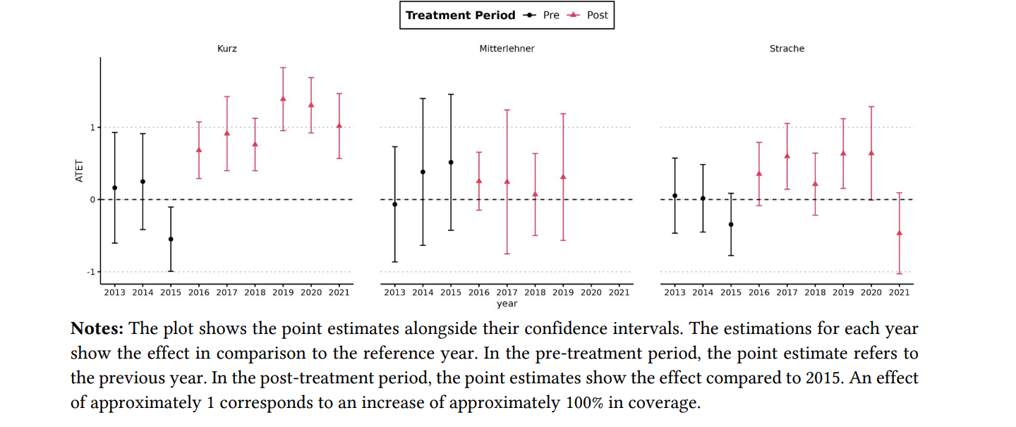
They implemented automated content analysis (using BERT) of political news articles from six prominent Austrian news outlets spanning 2012 to 2021 (n = 188,203) and adopted a difference-in-differences approach to scrutinize political actors’ visibility and favorability in news coverage for patterns indicative of the alleged serious breach of professional political and journalistic norms.

Methods
Used a German-language GottBERT model (Scheible et al., 2020) that they further fine-tuned for the task using publicly available data from the AUTNES Manual Content Analysis of the Media Coverage 2017 and 2019 (Galyga et al., 2022; Litvyak et al., 2022c)
Comparatively difficult task, but were able to reach a satisfactory F1-Score of 0.77 (precision = 0.77, recall = 0.77).
Findings
Our findings indicate a substantial increase in the news coverage of the former Austrian chancellor within the news outlet that is alleged to have received bribes.
In contrast, several other political actors did not experience similar shifts in visibility nor are similar patterns identified in other media outlets.
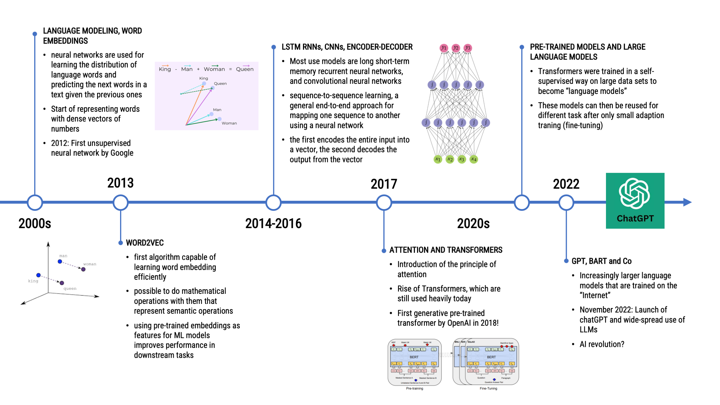
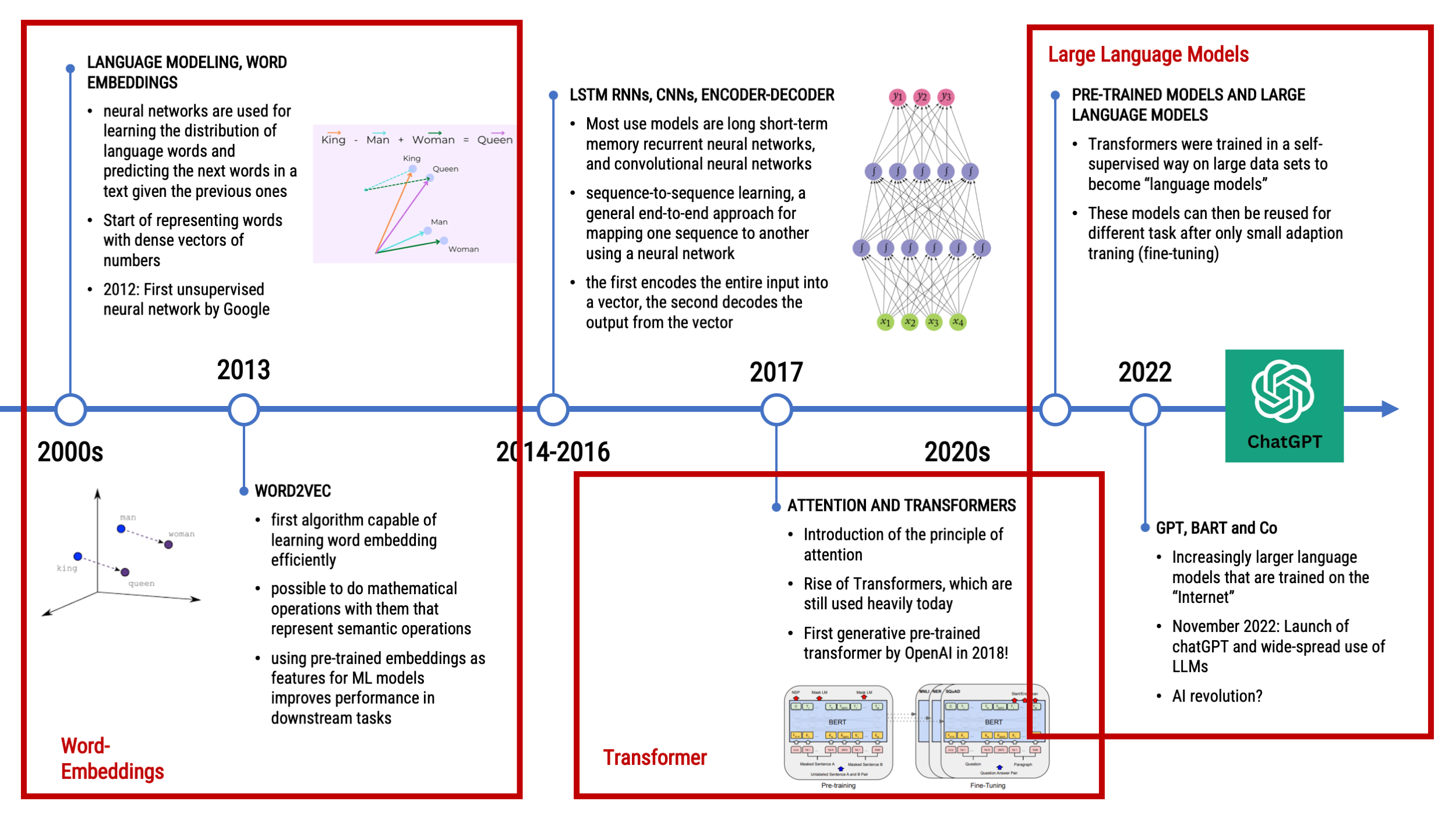
A Look Back at the Chronology of NLP
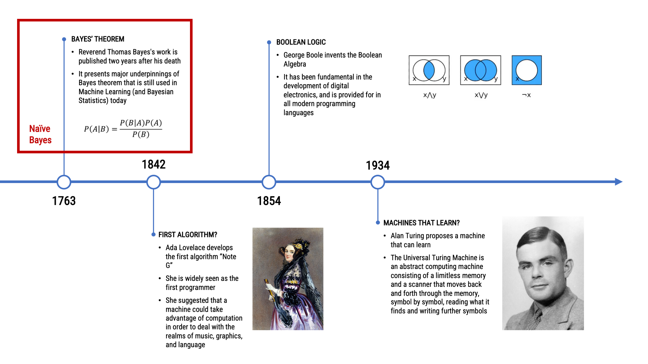
A Look Back at the Chronology of NLP
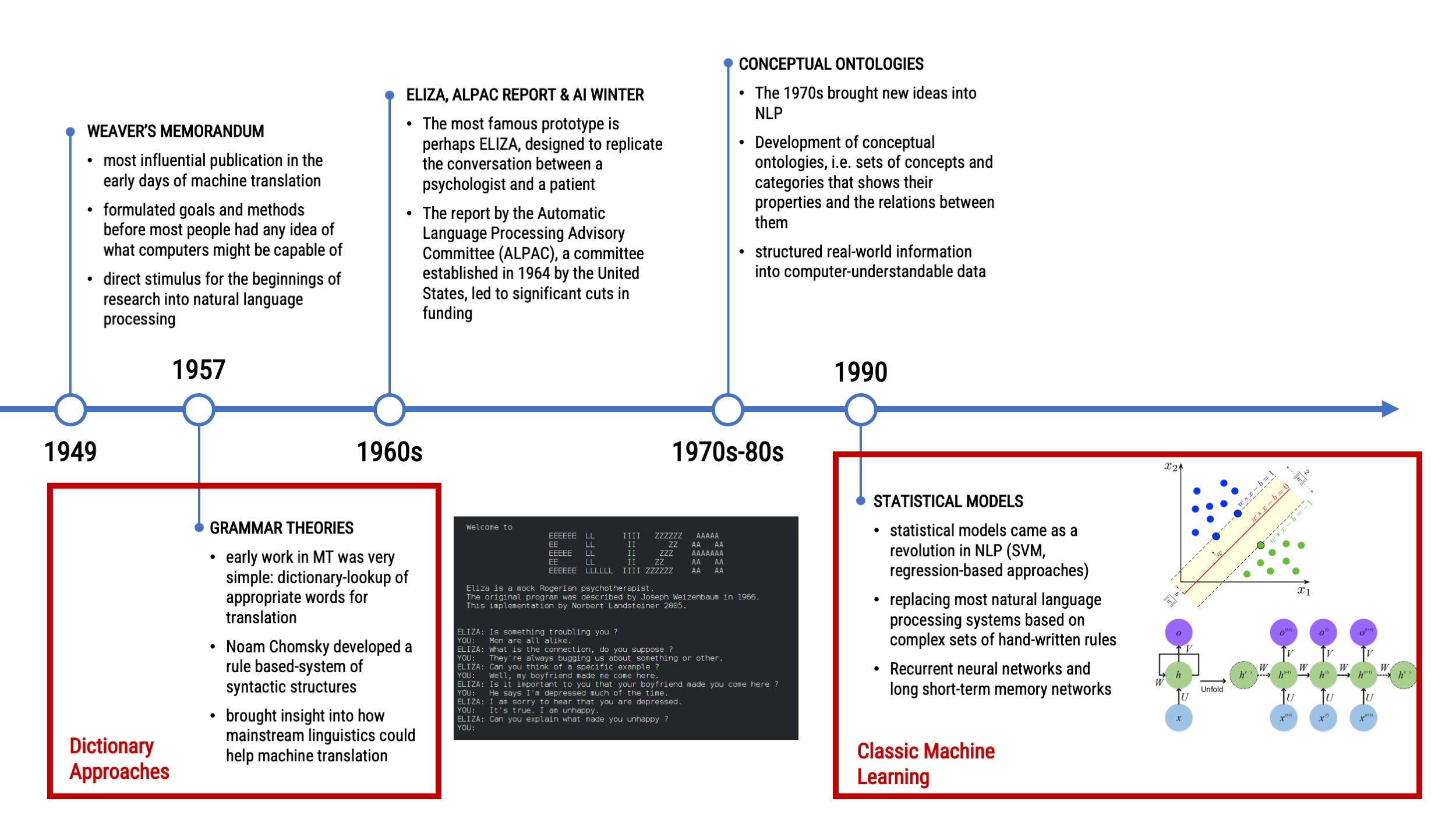
A Look Back at the Chronology of NLP
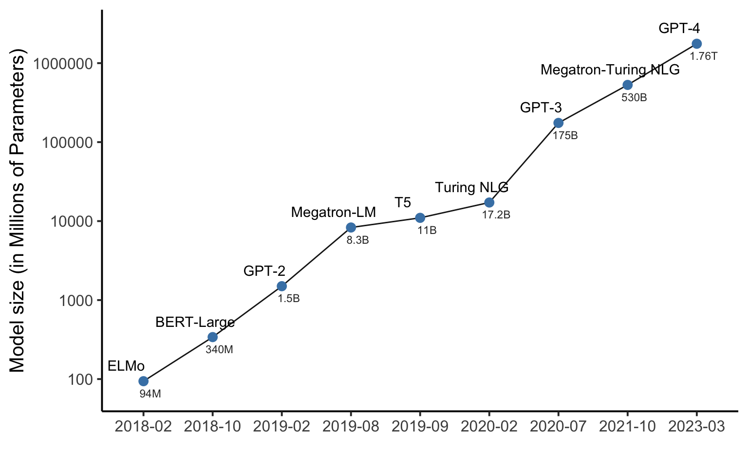
Explosion in model size?
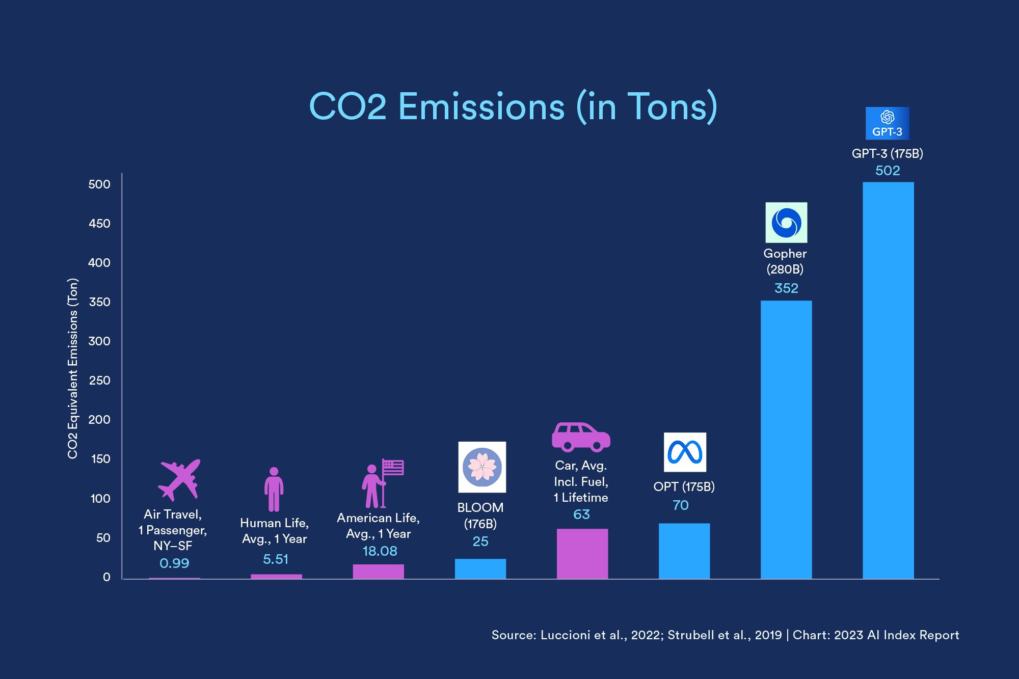
Environmental Impact
Conclusion
Advancement in NLP and AI are fast-paced; difficult to keep up
LLMs promise immense potential for communication research
Yet, large language models can contain biases or even hallucinate!
- Validation, validation, validation!


Example Exam Question (Open Format)
What does zero-shot learning refer to in the context of large language models?
In the context of large language models, zero-shot learning refers to the ability of a model to perform a task or make predictions on a set of classes or concepts that it has never seen or been explicitly trained on. Essentially, the model can generalize its knowledge to new, unseen tasks without specific examples or training data for those tasks.
In traditional machine learning, models are typically trained on a specific set of classes, and their performance is evaluated on the same set of classes during testing. Zero-shot learning extends this capability by allowing the model to handle tasks or categories that were not part of its training set.
In the case of large language models like GPT-3, which is trained on a diverse range of internet text, zero-shot learning means the model can understand and generate relevant responses for queries or prompts related to concepts it hasn’t been explicitly trained on. This is achieved through the model’s ability to capture and generalize information from the vast and varied data it has been exposed to during training.
![]()