Computational Analysis of Digital Communication

Week 4: Unsupervised Machine Learning - Topic Modeling

Dr. Philipp K. Masur

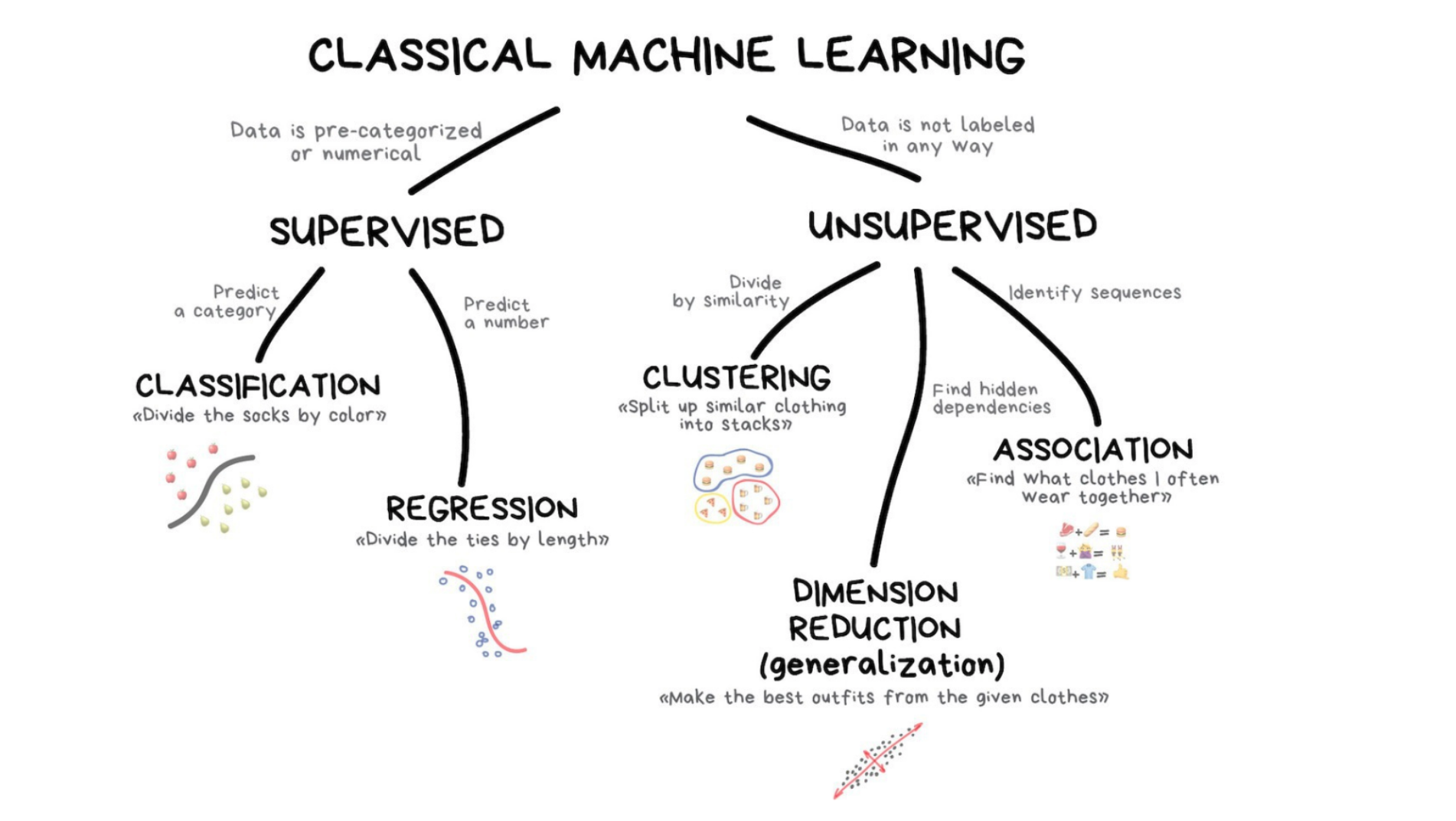
Supervised learning (last lecture)

• Algorithms build a model based on sample data, known as “training data”, in order to make predictions or decisions without being explicitly programmed to do so

• Combines the scalability of automatic coding with the validity of manual coding (requires pre-labeled data to train algorithm)

• Examples:

  • Supervised text classification, such as extending manual coding to large text corpora, sentiment analysis…
  • Pattern recognition: e.g., face recognition, spam filter,…

Unsupervised learning (this lecture)

• Algorithm detects clusters, patterns, or associations in data that has not been labeled previously, but researcher needs to interpret results

• Very helpful to make sense of new data (similar to cluster analysis or exploratory factor analysis)

• Examples:

  • Topic modeling: Extracting topics from unlabeled (text) data
  • Customer segmentation: Better understanding different customer groups around which to build marketing or other business strategies

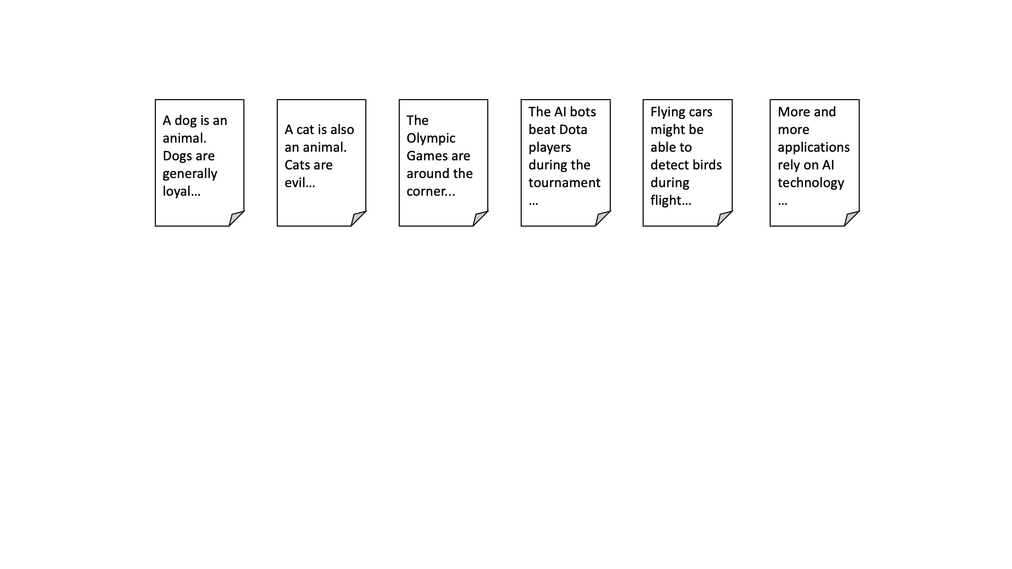
Computers can detect “topics”?

What are we trying to achieve?

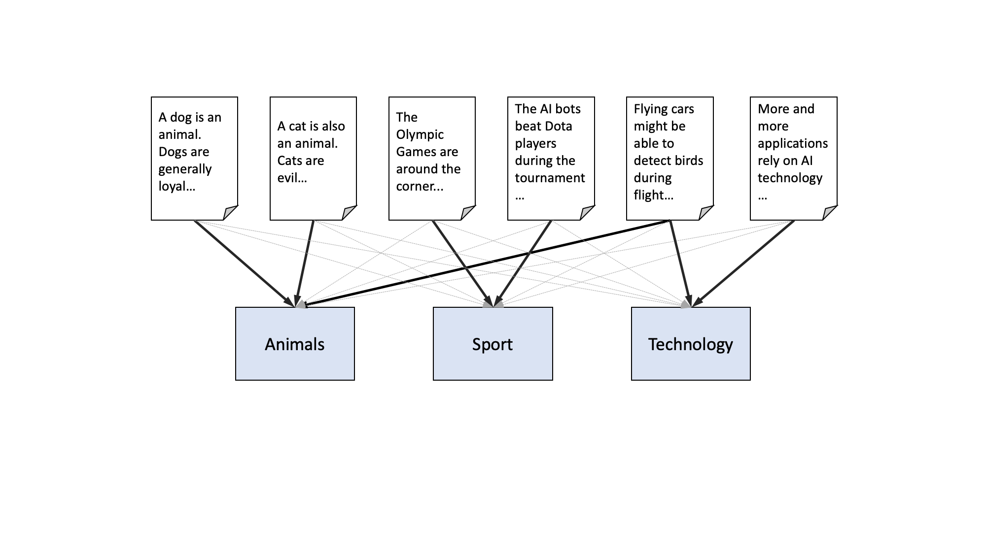
What topics can be extracted from the documents?

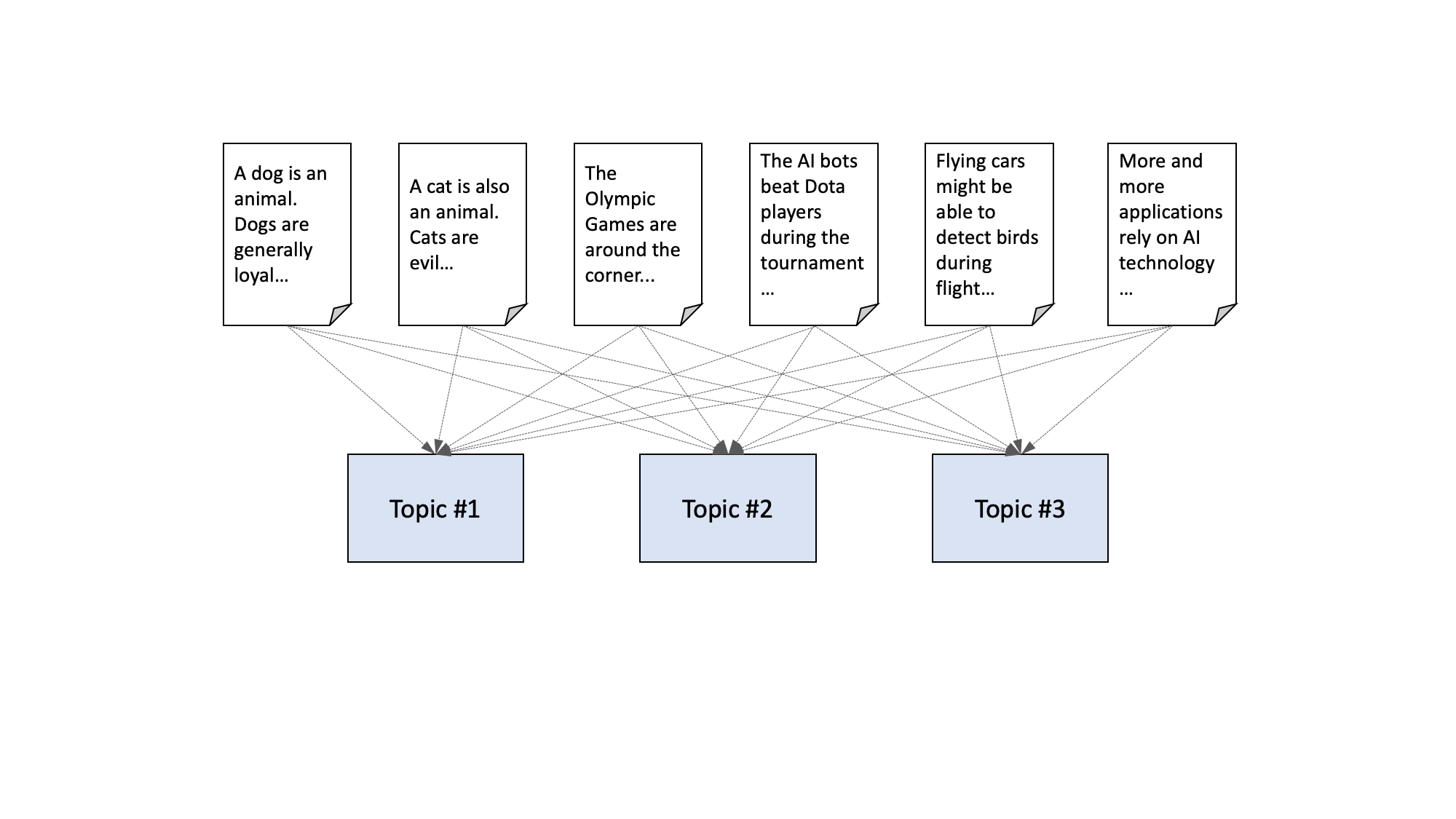
Easy for humans…

But the computer can only rely on words

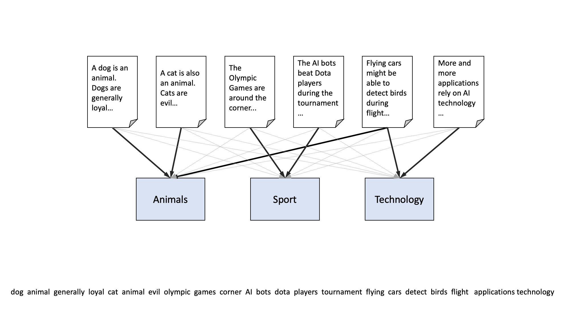
But each word may belong to a certain topic!

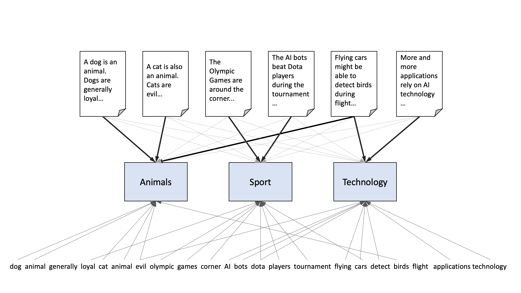
Goals of topic modeling

• Topic modeling is a method for unsupervised classification of documents

• It is somewhat similar to clustering on numeric data, which finds natural groups of items even when we’re not sure what we’re looking for

• The goal is to find a set of topics consisting of clusters of words that co-occur in these documents according to certain patterns

• However, the researchers must interpret the results of a topic model and there is usually more than one solution…

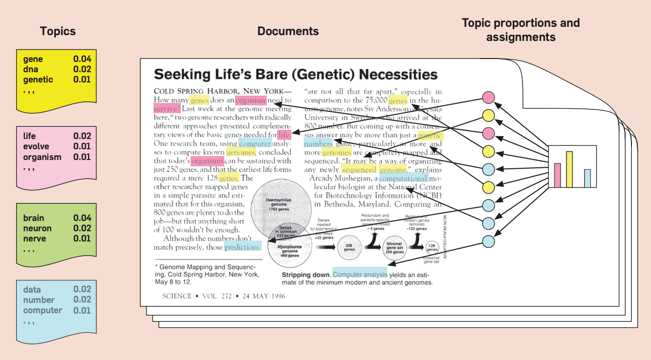
Blei, Ng, & Jordan, 2003

Why should we care?

• Topic models were originally developed as a text-mining tool and as such has wide applications in research that is based on understanding texts

• But topic models have applications in other fields such as bioinformatics and computer vision

  • can be used to detect structures in data such as genetic information
  • can also detect similaries in data based on images or networks

• More importantly, they are also used in various practical fields:

  • In news or content recommenders, which aim to suggest content based on similar topics
  • Used to power conversational agents (e.g., chatbots)
  • Spam filter (again!)
  • And many more…

Content of the lecture

1. What is topic modeling?

2. Topic Modeling as Dimensionality Reduction

3. Latent Dirichlet Allocation - LDA topic modeling

   • Basic Principles
   • Dirichlet Distribution
   • Gibbs Sampling
   • How to determine the right number of topics

4. (More) Examples from the literature

5. Conclusion and outlook

What is topic modeling?

Let’s start with an example

• Jacobi, Welbers & Van Atteveld (2016) analyzed the coverage of nuclear technology from 1945 to 2013 in the New York Times

• Overall, they analyzed 51,528 news stories (headline and lead): Way too much for human coding!

• Used Latent Dirichlet Allocation (LDA) topic modeling to extract topics

• They then analyzed the occurrence of topics over time

• It is a nice example of what topic modelling can and can’t do

Assumption of the model

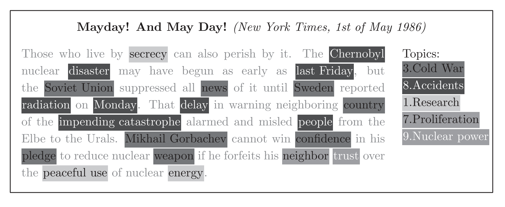
Characteristics of a topic model

This example highlights a number of interesting points about LDA topic modelling

1. The document is split between two main topics, Cold War and Nuclear Accidents: In a coding scheme forced to have a single topic per document, it would be very difficult to choose the dominant topic for this article.

2. Not all words are included in the analysis: Most are not used because they are non-substantive words such as determiners or prepositions (“the” or “it”), which the authors excluded, or because they are too rare (“Elbe”, “perish”) or too common (“have” but in this context also “nuclear”, since that was used to select the articles).

3. No a priori coding scheme was used by the computer, so the topics in this document were found completely automatically.

So what does a result of a Topic model look like?

• Typical table resulting from a topic model

• Contains most representative words per topic (in this case 10 topics)

• The authors then interpreted the outcome and labeled each topic accordingly

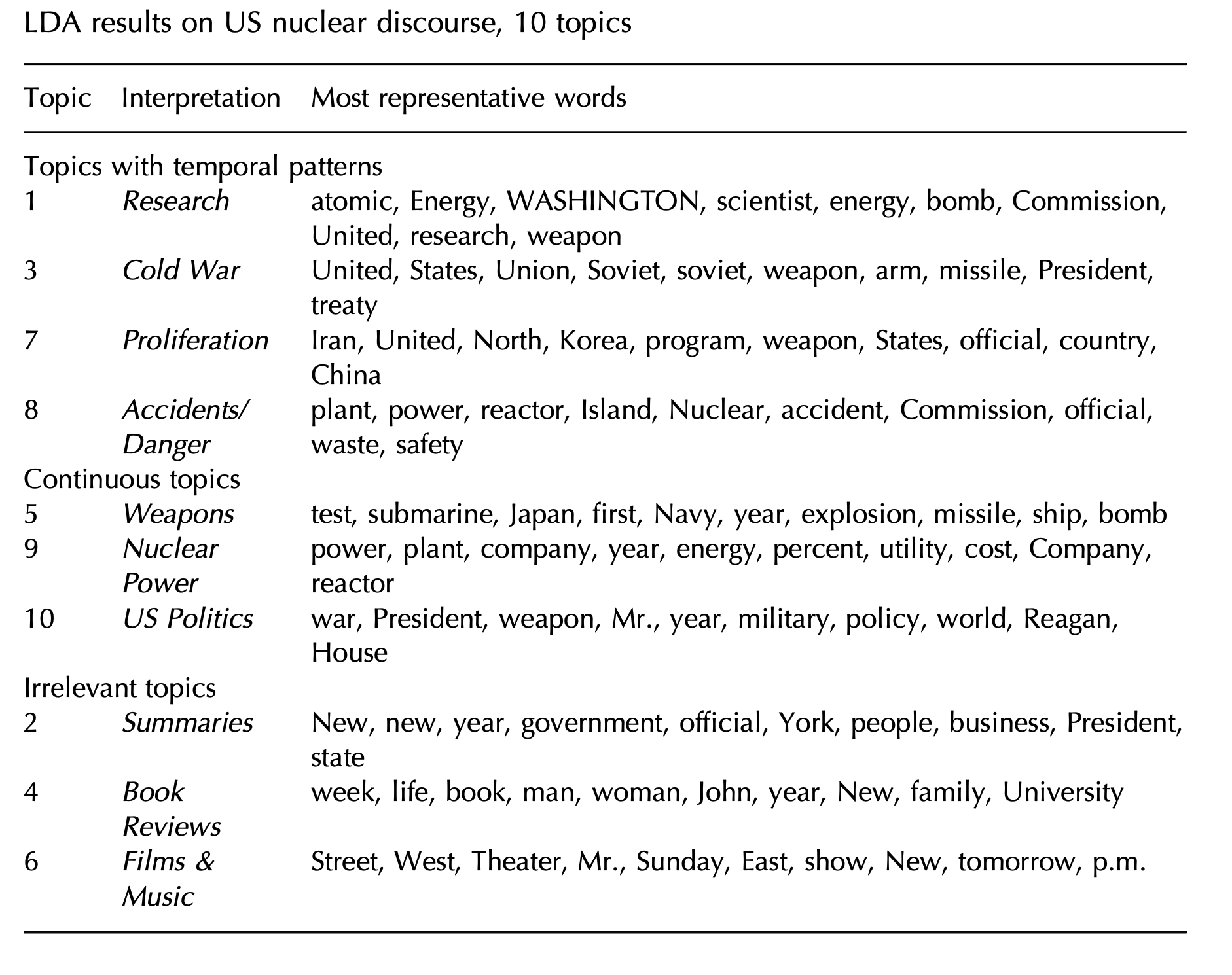
Using topics for substantive analyses

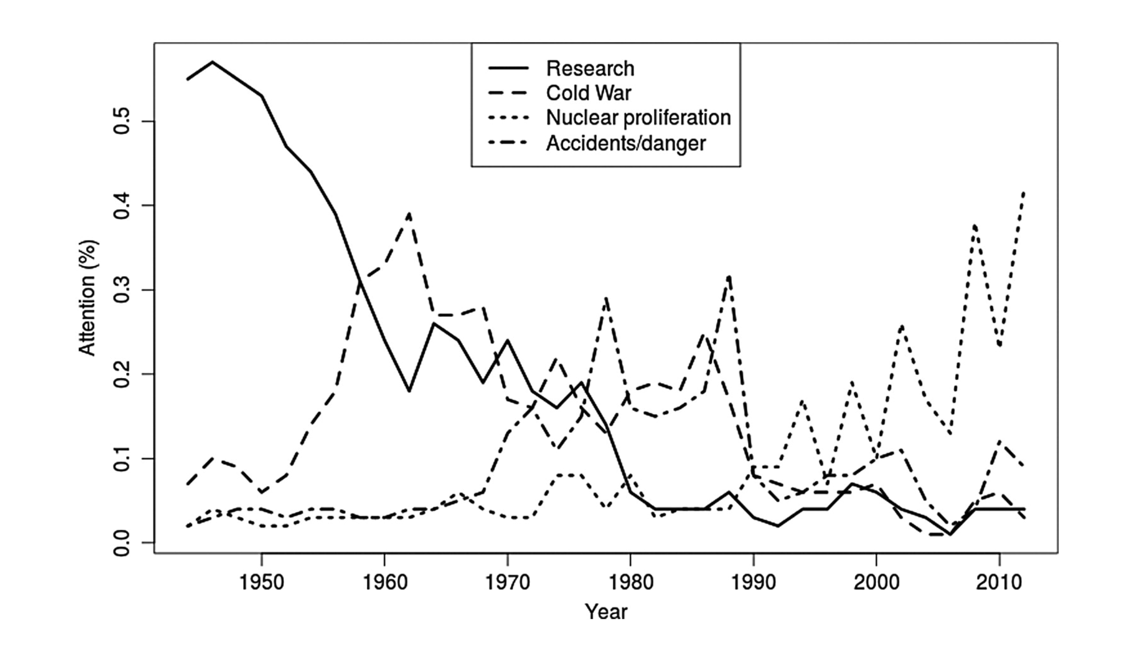
Topic Modeling as Dimensionality Reduction

Using factor or cluster analysis to extract topics?

• Problem: Texts are unstructured data and it is thus difficult to do standard statistical analysis with them

• Solution: Convert the texts into a document-term matrix, where documents represent cases and words are variables/characteristics of these cases

• Now we can use standard cluster/factor analysis techniques to reduce these dimensions?

Dimensionality reduction using PCA

# Loadin packages
library(tidyverse)
library(quanteda)

# Text examples
texts <- c("LDA is a topic model algorithm",
           "Topic modeling is an interesting example of LDA",
           "News algorithms are important in journalism",
           "Journalism is important for society",
           "Journalists use algorithms in their work")

# Text preprocessing
(dtm_factor <- texts %>%
  tokens(remove_punct = T) %>%
  tokens_remove(stopwords("en")) %>%
  dfm %>%
  as_tibble %>%
  select(-doc_id))

# A tibble: 5 × 15
    lda topic model algorithm modeling interesting example  news algorithms
  <dbl> <dbl> <dbl>     <dbl>    <dbl>       <dbl>   <dbl> <dbl>      <dbl>
1     1     1     1         1        0           0       0     0          0
2     1     1     0         0        1           1       1     0          0
3     0     0     0         0        0           0       0     1          1
4     0     0     0         0        0           0       0     0          0
5     0     0     0         0        0           0       0     0          1
# … with 6 more variables: important <dbl>, journalism <dbl>, society <dbl>,
#   journalists <dbl>, use <dbl>, work <dbl>

Dimensionality reduction using PCA

prcomp(dtm_factor, rank. = 2)

Standard deviations (1, .., p=5):
[1] 1.254104e+00 9.807140e-01 7.845689e-01 5.915016e-01 2.686400e-16

Rotation (n x k) = (15 x 2):
                   PC1         PC2
lda         -0.4297844  0.05075217
topic       -0.4297844  0.05075217
model       -0.1865506  0.01595800
algorithm   -0.1865506  0.01595800
modeling    -0.2432338  0.03479417
interesting -0.2432338  0.03479417
example     -0.2432338  0.03479417
news         0.1888600  0.13729363
algorithms   0.2970694 -0.28984625
important    0.3215750  0.37638771
journalism   0.3215750  0.37638771
society      0.1327150  0.23909408
journalists  0.1082094 -0.42713988
use          0.1082094 -0.42713988
work         0.1082094 -0.42713988

• Factor/Principal component analysis can reduce the number of columns (= reduce the dimensionality of the dataset)

• It assumes the manifest words are determined by (fewer) underlying latent factors

• In this simple example, it works to a certain degree, but we also see problems

Latent Semantic Analysis

• Latent Semantic Analysis assumes that words that are close in meaning will occur in similar pieces of text

• Singular value decomposition (SVD) is used to reduce the number of rows in a document-feature matrix while preserving the similarity structure among columns

• Overall, similar to factor analysis, but developed in the field of natural language processing

• Found to mimic (some) human generalizations and even errors

• Also problematic to interpret:

  • Negative values
  • Not robust to ambiguous terms and antonyms
  • No theoretical interpretation of mechanism

e.g. Deerwester et al., 1990

Preliminary conclusion

• Clustering, factor analysis, principal component analyis and its extension in the form of latent semantic analysis can all be used to reduce the dimensionality of a document-term matrix

• The resulting dimension may be a basis for extracting topics (after all it is words with loadings onto different factors = topics)

• Yet, there are several problems

  • Negative values difficult to interpret
  • The underlying model is hard to intepret

• These models are perhaps useful for understand which words load onto a topic, but they are less good at representing the distribution of topics in documents

Latent Dirichlet Allocation - LDA Topic Modeling

Latent Dirichlet Allocation - LDA topic modeling

• Evolution of Latent Semantic Analysis

• Is Based on generative statistical model that aligns with how articles or documents are written

  • It ‘assumes’ an author who…
  • chooses a mix of topics to write about.
  • For each word, s/he select one of the topics…
  • and then select a word from this topic.

• This basically results in a mixture model:

  • Words can be in multiple topics (→ deals with ambiguity)
  • Documents in multiple topics (→ deals with mixed content)
  • But skewed towards a couple of topics, depending on \(\alpha\) hyperparameter (more on this later)

Example for the generative model

Let’s assume that you are a journalist writing a 500 word news item.

1. You would choose one or more topics to write about, for example 70% healthcare and 30% economy.

2. For each word in the item, you randomly pick one of these topics based on their respective weight.

3. Finally, you pick a random word from the words associated with that topic, where again each word has a certain probability for that topic. For example, “hospital” might have a high probability for healthcare while “effectiveness” might have a lower probability but could still occur

Van Atteveldt, Trilling & Calderon, 2021

Intuitions behind LDA topic modelling

Blei et al., 2003

Sampling from the Dirichlet Distribution

• In topic modeling, we assume the following:

  • Every topic and document is a probability distribution (over words / topics resp.)
  • We wonder: How likely is word \(w\) in topic \(z\), or topic \(z\) in document \(d\)?
  • These distributions are themselves randomly drawn from the “dirichlet distribution” which yields multinomial distributions

• So, what is a “Dirichlet distribution”?

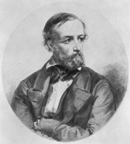
• Named after Peter Gustav Lejeune Dirichlet

• It is a family of continuous multivariate probability distributions parameterized by a vector \(\alpha\) of positive reals

• Can also be seen as a multivariate generalization of the beta distribution

Explaining a Dirichlet Distribution…

• You walk into the room for a get-to-gether (e.g., at a conference) and want to sit somewhere

• You are afraid to sit alone, so prefer a table with people

  • \(P(t_i) = n_i / sum(n)\)
  • To avoid \(sum(n)=0\) , every table starts at a baseline \(n = \alpha\)

• Everyone does the same as they enter

  • Empty tables stay empty, full tables keep getting more people proportionally
  • After many people have entered, an equilibrium emerges

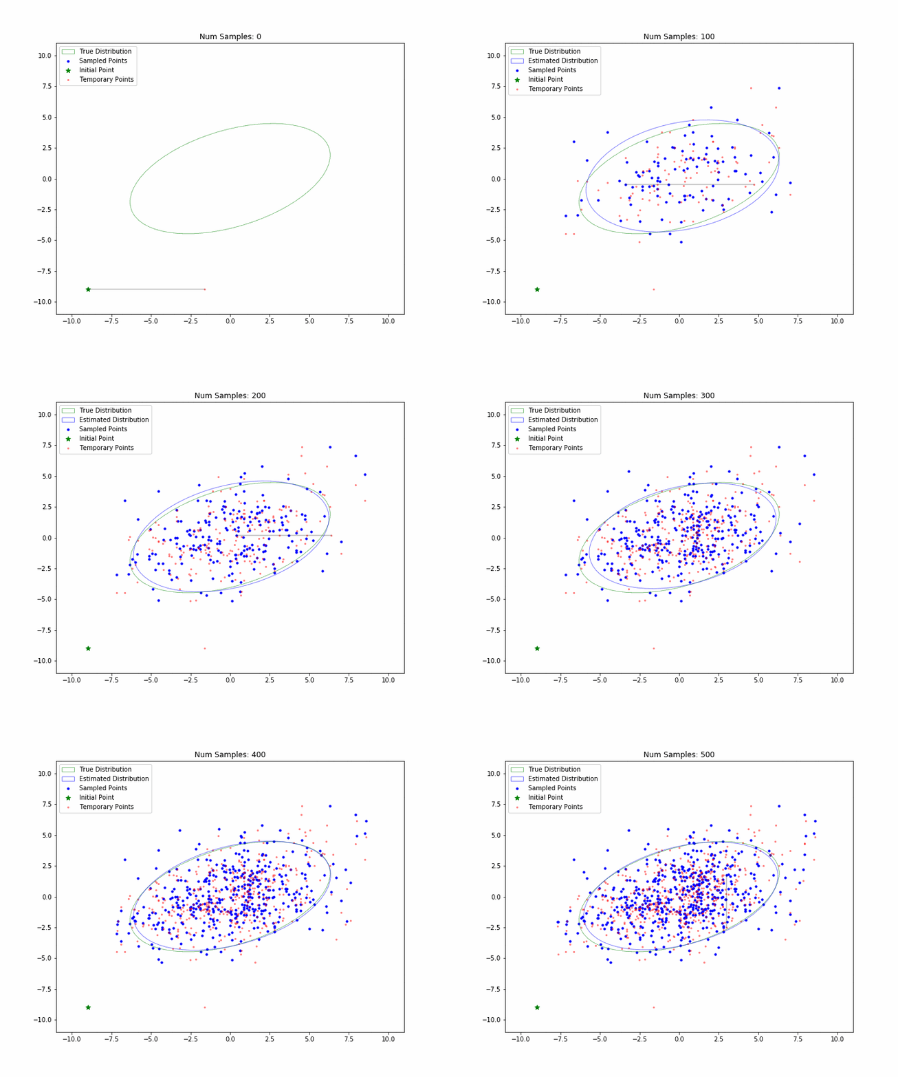
– Visual Demonstration of the Dirichlet Distribution –

Effect of the hyperparameter \(\alpha\)

• The restaurant converges to a multinomial distribution

  • E.g. the topics per document, or words per topic

• The initial number of people at the tables is the \(\alpha\) hyperparameter

  • Hyperparameter = ‘setting’/choice that affects how other parameters are estimated

• Intuitive effect of lower alpha:

  • initial choices of ‘customers’ have larger effect
  • likelier that a single table will get all participants

• Lower alpha = fewer topics per document

  • but means topic have to include more words / have more overlap, as each word needs to be assigned

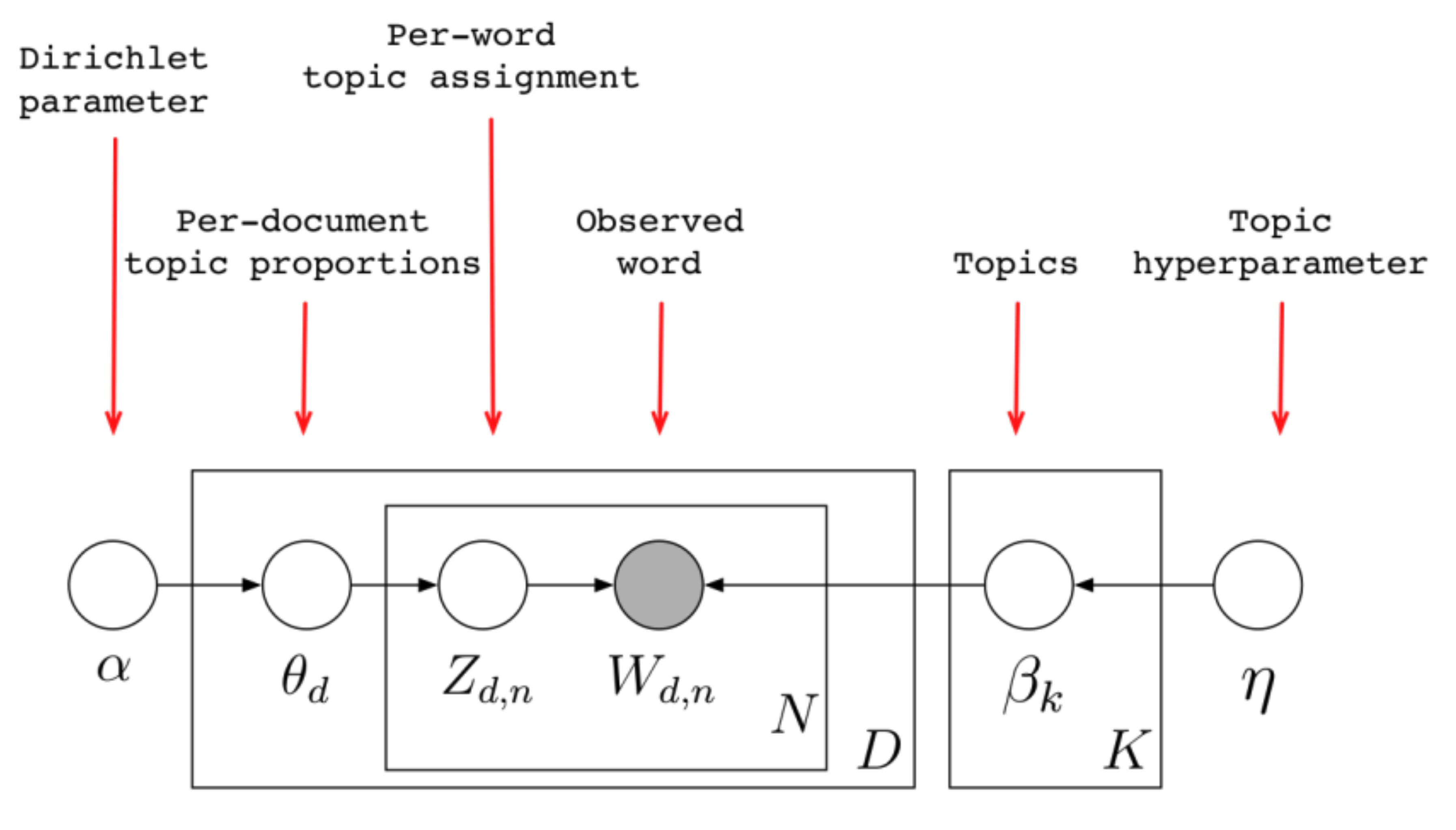
Plate notation of LDA

Blei et al., 2003

For each document d:

• Draw random topic proportions \(\theta_d\)
• For each word n in document d:
  • Draw a single topic \(Z\) from \(\theta_d\)
  • Draw a word \(W\) from \(\beta_z\)

\(\beta_k\) and \(\theta_d\) are drawn from \(Dir(\alpha)\) and thus not observed directly

Question: How can we determine these parameters?

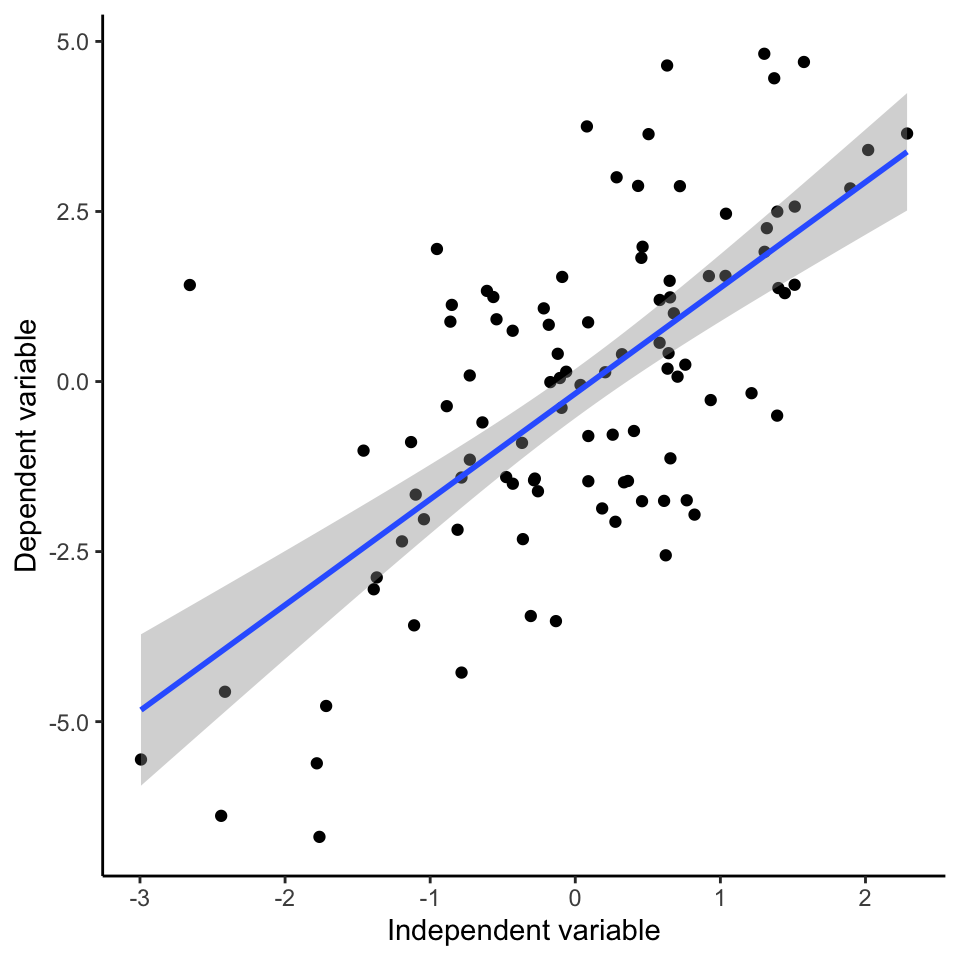
Think about a regression analysis…

• A regression analysis aims to predict \(x\) from \(y\)

• It assumes a linear relationship between the two variables that can be expressed as

\(y_i = \beta_0 + \beta_1*x_i + e_i\)

• Similar to the topic model, we have \(x\) and \(y\), but we don’t actually have the parameter of interest: \(\beta_0\), and \(\beta_1\)

• Through methods such as ordinary least squares, we try to find the value of the \(\beta\)’s that minimize the sum of squared errors

Reverse-Engineering the Generative Model

• The generative model assumes we know the parameters and want to find the words

• But similar to the regression analysis, our challenge is the opposite:

  • We know the actual words in the corpus
  • How can we find out the parameters of the model the explain their occurence?

• Task: Find the parameters that maximize the likelihood of the corpus

• Unfortunately, there is no analytic solution

  • Contrast with e.g. SVD and OLS that can be computed directly
  • Similar to multilevel models, this is not the case for LDA

• Need to do iterative approximation of best solution

Gibbs Sampling in LDA

• refers to a Markov chain Monte Carlo (MCMC) algorithm for obtaining a sequence of observations which are approximated from a specified multivariate probability distribution

• Suppose you know the topics of all words except for one word \(w\)

• This new word \(w\) is the new guest entering the restaurant

  • Pick a topic within the document proportional to existing topics in the document (plus alpha)
  • Pick a topic for the word proportional to existing topics for this word (plus eta)

• This gives a joint probability for all topics for this word

Iterative Gibbs Sampling

1. Start with random assignments of topics to words

2. For each word \(w\) in document \(d\)

   • Compute proportion of topics in word and document (disregarding \(w\) itself)
   • Compute probability of each topic \(z\) given those proportions
   • Pick a new topic from that probability
   • Update proportions for next iteration

3. Repeat from 2 until converged

• This may sounds complicated and we won’t dive deeper into this topic.

• However, if you are interested in how this works in detail, check out the blog post “LDA under the hood” by A. Brook!

Let’s look at an Example in R

library(quanteda)
library(quanteda.textplots)
library(tidyverse)
library(topicmodels)

s1 <- read_csv("data/science articles/train.csv") %>%
  select(id = ID, title = TITLE, abstract = ABSTRACT) %>%
  slice(1:5000) # Make it a little smaller to run faster

head(s1)

# A tibble: 6 × 3
     id title                                                           abstract
  <dbl> <chr>                                                           <chr>   
1     1 Reconstructing Subject-Specific Effect Maps                     "Predic…
2     2 Rotation Invariance Neural Network                              "Rotati…
3     3 Spherical polyharmonics and Poisson kernels for polyharmonic f… "We int…
4     4 A finite element approximation for the stochastic Maxwell--Lan… "The st…
5     5 Comparative study of Discrete Wavelet Transforms and Wavelet T… "Fourie…
6     6 On maximizing the fundamental frequency of the complement of a… "Let $\…

Text Preprocessing and DTM

dtm <- s1 %>%
  corpus(text = "abstract") %>%
  tokens(remove_punct = T, remove_numbers = T) %>%
  tokens_remove(stopwords("en")) %>%
  tokens_select(min_nchar = 2) %>%
  dfm %>%
  dfm_trim(min_termfreq = 5)
dtm

Document-feature matrix of: 5,000 documents, 9,238 features (99.33% sparse) and 2 docvars.
       features
docs    predictive models allow subject-specific inference analyzing disease related alterations neuroimaging
  text1          2      3     1                4         4         1       3       1           1            2
  text2          0      0     0                0         0         0       0       0           0            0
  text3          0      0     0                0         0         0       0       0           0            0
  text4          0      0     0                0         0         0       0       0           0            0
  text5          0      0     0                0         0         0       0       0           0            0
  text6          0      0     0                0         0         0       0       0           0            0
[ reached max_ndoc ... 4,994 more documents, reached max_nfeat ... 9,228 more features ]

Text preprocessing

• Text preprocessing is more important for topic modeling than for other machine learning approaches

• For example keeping stopwords will lead to non-sensical “topics” because they co-occur so often

• Stemming or lemmatizing will streamline words and thereby improve coherence between topics.

• We want to make sure that the model focuses on those words that really tell something about the topic

• Text preprocessing stepts are often pivotal for the interpretability of the resulting topics

Estimating a topic model in R

library(topicmodels)

# Convert dtm to topicmodels' specific format
dtm <- convert(dtm, to = "topicmodels") 

# Set seed to make it reproducible
set.seed(1)

# Fit topic model
m <- LDA(dtm, 
         method = "Gibbs", 
         k = 6,  
         control = list(alpha = 0.1))
m

A LDA_Gibbs topic model with 6 topics.

• We need to chose the sampling method: usually Gibbs sampling

• We need to specify the number of topics (\(k\)) a priori, but we can of course try out different solutions

• We can set the alpha parameter for the Dirichlet distribution

Inspecting LDA results

By using the function terms(), we can have a look at the most probable words in each of the six topics:

terms(m, 15) %>%
  as_tibble

# A tibble: 15 × 6
   `Topic 1`    `Topic 2`   `Topic 3`    `Topic 4`   `Topic 5` `Topic 6` 
   <chr>        <chr>       <chr>        <chr>       <chr>     <chr>     
 1 algorithm    data        observations learning    show      can       
 2 problem      can         data         data        prove     magnetic  
 3 data         system      mass         network     also      phase     
 4 model        paper       galaxies     networks    graph     energy    
 5 method       systems     stars        neural      mathbb    model     
 6 can          network     find         model       paper     quantum   
 7 methods      using       star         can         group     state     
 8 paper        analysis    can          deep        space     field     
 9 show         based       using        training    study     states    
10 results      time        emission     method      graphs    system    
11 distribution different   stellar      models      given     dynamics  
12 models       model       present      using       result    spin      
13 approach     information galaxy       propose     results   two       
14 optimization used        two          performance finite    systems   
15 time         control     results      methods     set       properties

Question: What topics do these wordlists stand for?

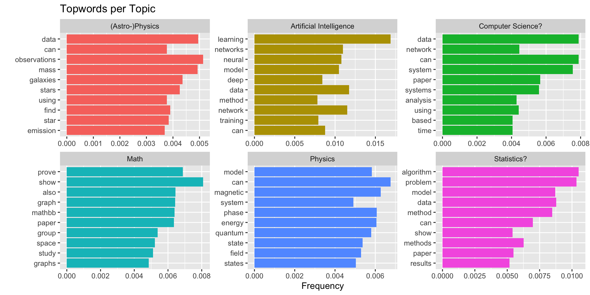
Top words in each topic

But because we gain a probability with which a word is in a topic, we can also look at these probabilities per word per topic:

topic <- 3
words <- posterior(m)$terms[topic, ]
topwords <- sort(words, 
                 decreasing = T) %>%
  head(n = 50)
head(topwords, 10) %>% 
  as.data.frame

                       .
observations 0.005133322
data         0.004952844
mass         0.004927061
galaxies     0.004359843
stars        0.004256713
find         0.003895756
star         0.003844190
can          0.003766843
using        0.003766843
emission     0.003689495

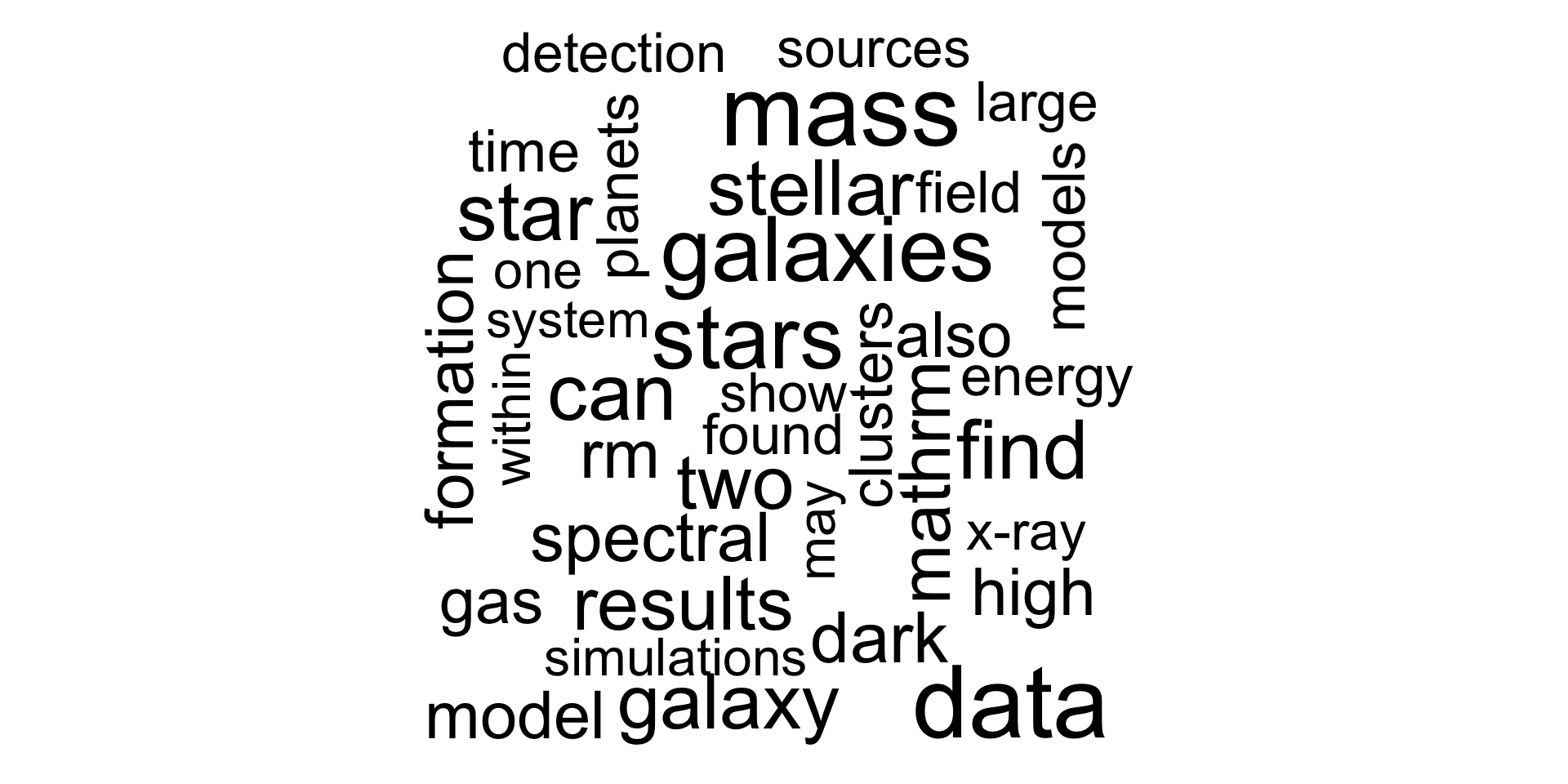
library(wordcloud)
wordcloud(names(topwords), topwords)

Alternative visualization

Probabilites of topics per document

• From the topic model, we can extract a table that shows us the probabilities of a topic being written about in the different texts (bear in mind, several topics can be in one text)

• We see for example, that there is a high probability of the text 7 being about topic 3 (astrophysics)

posterior(m)$topics %>% 
  as.data.frame() %>%
  rownames_to_column("doc") %>%
  as_tibble

# A tibble: 5,000 × 7
   doc        `1`      `2`     `3`      `4`      `5`     `6`
   <chr>    <dbl>    <dbl>   <dbl>    <dbl>    <dbl>   <dbl>
 1 text1  0.234   0.000569 0.0177  0.695    0.000569 0.0518 
 2 text2  0.00198 0.00198  0.00198 0.753    0.239    0.00198
 3 text3  0.00224 0.00224  0.00224 0.00224  0.989    0.00224
 4 text4  0.391   0.00162  0.00162 0.00162  0.375    0.229  
 5 text5  0.341   0.00136  0.00136 0.654    0.00136  0.00136
 6 text6  0.0105  0.000956 0.0583  0.000956 0.919    0.0105 
 7 text7  0.00198 0.0415   0.951   0.00198  0.00198  0.00198
 8 text8  0.00150 0.00150  0.00150 0.0465   0.00150  0.947  
 9 text9  0.0179  0.00162  0.229   0.00162  0.00162  0.748  
10 text10 0.00124 0.373    0.00124 0.212    0.100    0.311  
# … with 4,990 more rows

Is text 7 really about astrophysics?

s1 %>%
  filter(id == 7) %>%
  select(abstract) %>%
  as.character()

[1] "We observed the newly discovered hyperbolic minor planet 1I/`Oumuamua (2017\nU1) on 2017 October 30 with Lowell Observatory's 4.3-m Discovery Channel\nTelescope. From these observations, we derived a partial lightcurve with\npeak-to-trough amplitude of at least 1.2 mag. This lightcurve segment rules out\nrotation periods less than 3 hr and suggests that the period is at least 5 hr.\nOn the assumption that the variability is due to a changing cross section, the\naxial ratio is at least 3:1. We saw no evidence for a coma or tail in either\nindividual images or in a stacked image having an equivalent exposure time of\n9000 s.\n"

Probabilites of topics per document

Let’s check out another one: text 2 seems to be primarily about topic 4 (machine learning?):

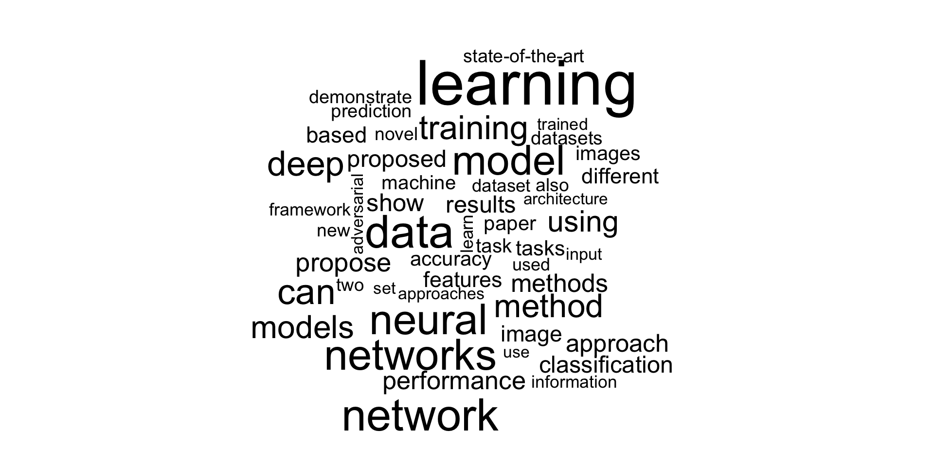
topic <- 4
words <- posterior(m)$terms[topic, ]
topwords <- head(sort(words, decreasing = T), n=50)
wordcloud(names(topwords), topwords)

s1 %>%
  filter(id == 2) %>%
  select(abstract) %>%
  as.character()

[1] "Rotation invariance and translation invariance have great values in image\nrecognition tasks. In this paper, we bring a new architecture in convolutional\nneural network (CNN) named cyclic convolutional layer to achieve rotation\ninvariance in 2-D symbol recognition. We can also get the position and\norientation of the 2-D symbol by the network to achieve detection purpose for\nmultiple non-overlap target. Last but not least, this architecture can achieve\none-shot learning in some cases using those invariance.\n"

Substantive analyses

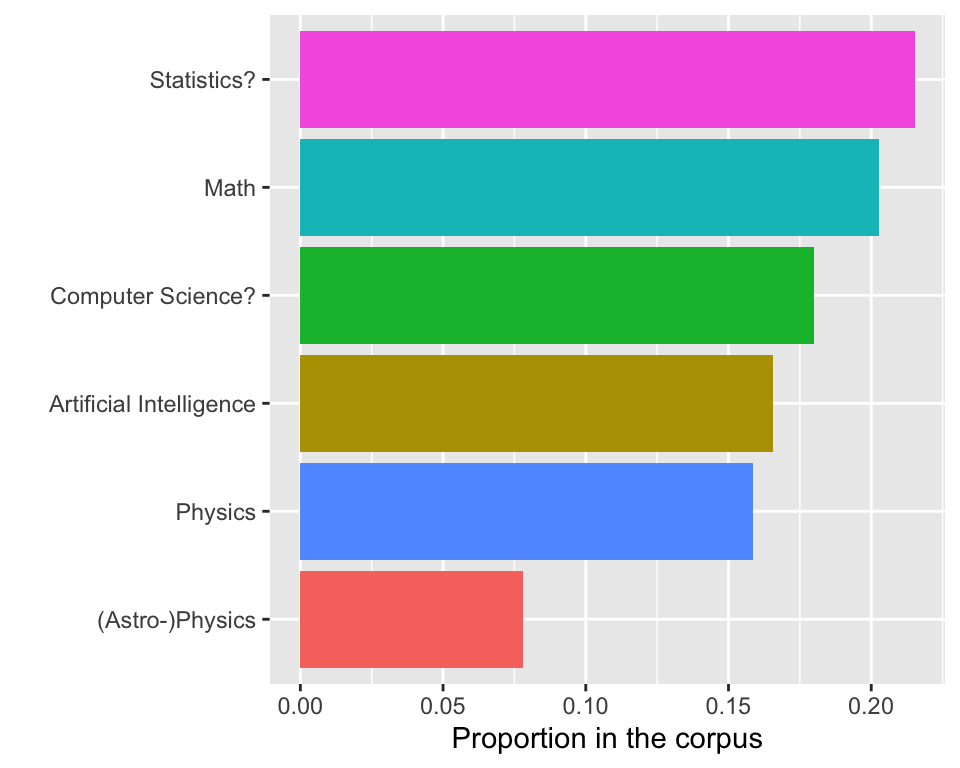
Depending on the research questions, we now may for example want to describe the topic prevalence in the corpus.

(table <-  posterior(m)$topics %>%
  as.data.frame %>%
  rownames_to_column("docs") %>%
  gather(topic, value, -docs) %>%
  as_tibble %>%
  arrange(docs, value))

# A tibble: 30,000 × 3
   docs   topic    value
   <chr>  <chr>    <dbl>
 1 text1  2     0.000569
 2 text1  5     0.000569
 3 text1  3     0.0177  
 4 text1  6     0.0518  
 5 text1  1     0.234   
 6 text1  4     0.695   
 7 text10 1     0.00124 
 8 text10 3     0.00124 
 9 text10 5     0.100   
10 text10 4     0.212   
# … with 29,990 more rows

Visualization of topic prevalence

• Bear in mind that this is not the proportion of articles that are about this topic!

• It is the overall proportion of the topic in the corpus given that articles can be about several topics

table %>%
  group_by(topic) %>%
  summarize(prop = mean(value)) %>%
  mutate(topic = recode(topic, 
         "1" = "Statistics?", 
         "2" = "Computer Science?", 
         "3" = "(Astro-)Physics", 
         "4" = "Artificial Intelligence", 
         "5" = "Math", 
         "6" = "Physics")) %>%
  ggplot(aes(x = fct_reorder(topic, prop), 
             y = prop, fill = topic)) +
  geom_col() +
  coord_flip() +
  theme(legend.position = "none") +
  labs(x = "", 
       y = "Proportion in the corpus")

Validation

• The first step after fitting a model is inspecting the results and establishing face validity

• Top words per topic are a good place to start, but one should also look at the top documents per topic to better understand how words are used in context.

• Also, it is good to inspect the relationships between topics and look at documents that load high on multiple topics to understand the relationship

• If one using topic models in a more confirmatory manner, e.g., the topics should match some sort of predefined categorization, you should use regular gold standard techniques for validation:

  • code a sufficiently large random sample of documents with your predefined categories, and test whether the LDA topics match those categories (compute accuracy, precision, recall, F1-score)
  • In general, however, in such cases it is a better idea to use a dictionary or supervised analysis technique as topic models often do not exactly capture our categories

Choosing the right number of topics

• Topic models such as LDA allow you to specify the number of topics in the model

  • This is a nice thing because it allows you to adjust the granularity of what topics measure: between a few broad topics and many more specific topics.
  • But it begets the question what the best number of topics is.

• The short and perhaps disappointing answer is: The best number of topics does not exist

  • there is no singular idea of what a topic even is is
  • it depends on what you are interested in: e.g., if you want know what a corpus is about, you want to have a limited number of topics that provide a good representation of overall themes

• But even if the best number of topics does not exist, some values for k (i.e. the number of topics) are better than others.

  • If we use too few topics, there will be variance in the data that is not accounted for,
  • If you use too many topics you will overfit and get topics that are not interesting

How well does our model fit the data?

• One approach to the “best” number of topics is to check which model best predicts the data

• This is comparable to goodness-of-fit measures for statistical models (e.g., log likelihood, CFI, etc.)

• For LDA topic models, a commonly usd indicator is perplexity (Blei, Ng, & Jordan, 2003), where lower perplexity indicate better predictin/fit

• To calculate perplexity, we follow an already known procedure (last lecture!):

  • We first train an LDA model on a portion of the data
  • Then, we model is evaluatd using the held-out portion of the data
  • This procedure is repeated for models with different numbers of topics so that it becomes clear which one leads to the lowest perplexity

Calculating perplexity in R

• We first have to split up our data into data for training and testing the model

• This way we prevent overfitting the model

• Here we’ll use 75% for training, and held-out the remaining 25% for test data.

# Split sample
train <- sample(rownames(dtm), nrow(dtm) * .75)
dtm_train <- dtm[rownames(dtm) %in% train, ]
dtm_test <- dtm[!rownames(dtm) %in% train, ]

• Then, we train the model and then, we calculate the perplexity by testing the model on the test data

m_train <- LDA(dtm_train, method = "Gibbs", k = 6,  control = list(alpha = 0.01))
perplexity(m, dtm_test)

[1] 1977.736

Estimating several model and perplexity scores

• A single perplexity score is not really useful as we have nothing to compare it against

• Instead, we calculate the perplexity score for models with different parameters, to see how this affects the perplexity

p <- data.frame(k = c(3,6,12,24,48,96),
                perplexity = NA)

## loop over the values of k in data.frame p 
for (i in 1:nrow(p)) {
  # calculate perplexity for the given value of k
  m <- LDA(dtm_train, 
           method = "Gibbs", 
           k = p$k[i],  
           control = list(alpha = 0.01))
  # store result in our data.frame
  p$perplexity[i] = perplexity(m, dtm_test)
}

# Output
p

   k perplexity
1  3   2665.177
2  6   2417.928
3 12   2170.333
4 24   1991.856
5 48   1854.943
6 96   1800.028

Visualizing a perplexity curve

• Technically, the best fitting model is the one with the lowest perplexity score

  • But this will always be a model with a lot of topics!

• If we want to use topic modelling for bottom-up inductive analyses of text corpora, we need to look for a “knee” in the plot

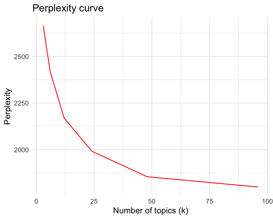
ggplot(p, aes(x = k, y = perplexity)) + 
  geom_line(color = "red") +
  theme_minimal() +
  labs(x = "Number of topics (k)",
       y = "Perplexity",
       title = "Perplexity curve")

New model with 12 topics

m2 <- LDA(dtm, 
         method = "Gibbs", 
         k = 12,  
         control = list(alpha = 0.1))
terms(m2, 10)

      Topic 1        Topic 2     Topic 3     Topic 4       Topic 5       
 [1,] "mass"         "method"    "network"   "system"      "data"        
 [2,] "observations" "using"     "networks"  "systems"     "model"       
 [3,] "galaxies"     "images"    "model"     "can"         "models"      
 [4,] "stars"        "image"     "can"       "performance" "distribution"
 [5,] "find"         "signal"    "dynamics"  "paper"       "method"      
 [6,] "star"         "can"       "different" "code"        "can"         
 [7,] "stellar"      "noise"     "nodes"     "power"       "methods"     
 [8,] "galaxy"       "based"     "models"    "network"     "estimation"  
 [9,] "emission"     "detection" "time"      "data"        "results"     
[10,] "can"          "imaging"   "social"    "memory"      "used"        
      Topic 6       Topic 7        Topic 8         Topic 9       Topic 10 
 [1,] "data"        "algorithm"    "control"       "magnetic"    "mathbb" 
 [2,] "analysis"    "problem"      "system"        "phase"       "show"   
 [3,] "research"    "algorithms"   "can"           "energy"      "prove"  
 [4,] "can"         "problems"     "approach"      "field"       "group"  
 [5,] "paper"       "optimization" "learning"      "spin"        "also"   
 [6,] "using"       "can"          "policy"        "quantum"     "mathcal"
 [7,] "information" "show"         "reinforcement" "state"       "paper"  
 [8,] "users"       "number"       "model"         "states"      "study"  
 [9,] "study"       "optimal"      "environment"   "temperature" "groups" 
[10,] "different"   "matrix"       "using"         "surface"     "finite" 
      Topic 11   Topic 12   
 [1,] "learning" "equation" 
 [2,] "neural"   "solutions"
 [3,] "model"    "equations"
 [4,] "network"  "system"   
 [5,] "deep"     "theory"   
 [6,] "data"     "can"      
 [7,] "training" "method"   
 [8,] "networks" "numerical"
 [9,] "models"   "systems"  
[10,] "can"      "nonlinear"

Example from the literature

What communication scholars write about

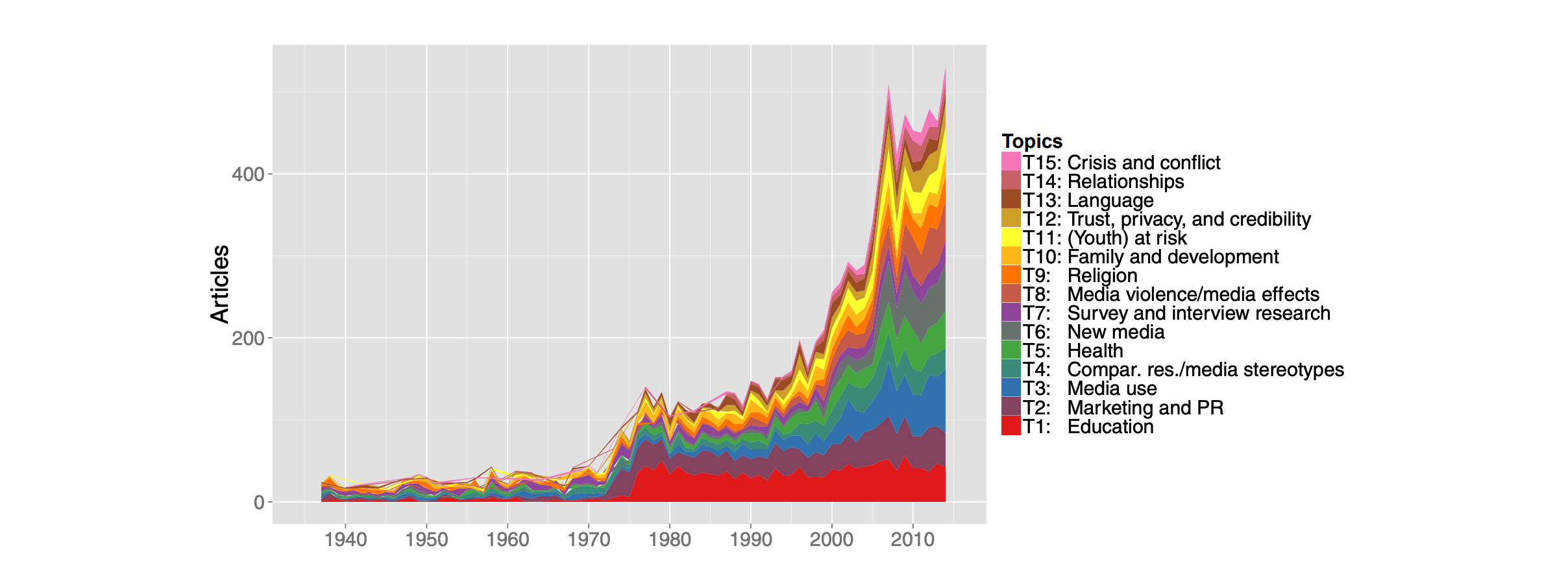
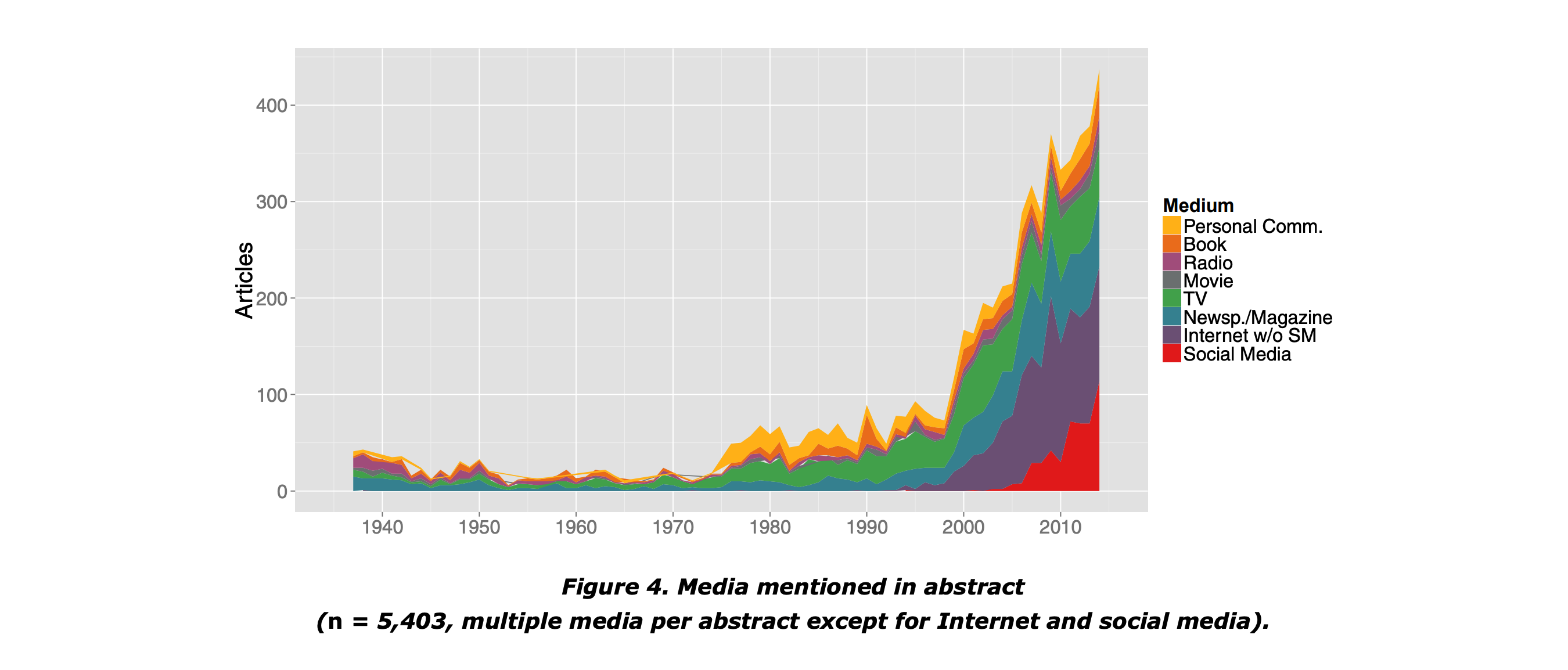
• Günther and Domahidi (2017) used LDA topic modeling to get an overview of research topics in 80 years of communication research

• Documents were 15,000 abstracts from academic journals

• To find a reasonable value k (number of topics), they ran 40 topic models with k = 5 to k = 200 and systematically compared them: The final model hat 145 topics

• For each document (abstract), they selected the two topics with the highest probability (minimum probability was .1)

• To ensure a meaningful interpretation, the authors validated the labels of the inferred topics by manually checking publications from every decade that contained the topic with high probability.

Core topics in communication research

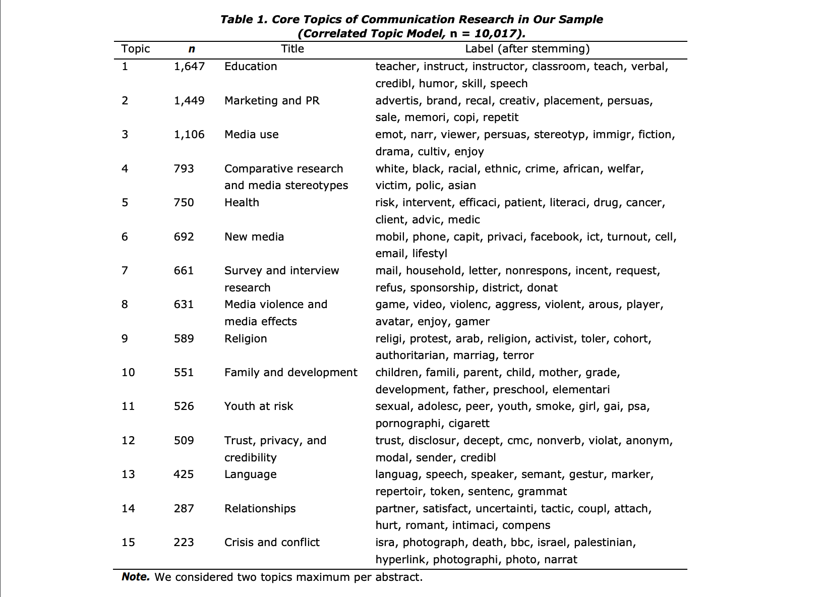
Evolution of topics over time

Type of media researched over time

Conclusions and outlook

What is the state of the art?

• LDA is still one of the most used approaches to topic modeling and performs well in many circumstances

• Yet, there are many new approaches including e.g., structural topic modeling (see R package stm; Roberts et al., 2019)

  • an extension of LDA that allow us to explicitly model text metadata such as date or author as covariates of the topic prevalence and/or topic words distributions
  • Text contextual information into account!

• Recent advances have been made by using pre-trained transformer-based language models (BERT, BERTopic; Grootendorst, 2022)

  • generates document embedding with pre-trained transformer-based language models
  • clusters these embeddings
  • generates topic representations with the class-based TF-IDF procedure.

Conclusion

• Topic Modeling reduces the dimensionality of a document-term matrix by clustering words and documents into “latent” topics

• Interpretation of resulting “topic solutions” must be done by the researcher (face validity)

• LDA is driven by the Dirichlet process that yields distributions

  • skewed towards few topics, but controllable with alpha parameter

• Gibbs sampling is a non-deterministic way to fit LDA models

Thank you for your attention!

Required Reading

Günther, E. , & Domahidi, E. (2017). What Communication Scholars Write About: An Analysis of 80 Years of Research in High-Impact Journals. International Journal of Communication 11(2017), 3051–3071

Jacobi,C., van Atteveldt, W. & Welbers, K. (2016) Quantitative analysis of large amounts of journalistic texts using topic modelling. Digital Journalism, 4(1), 89-106, DOI: 10.1080/21670811.2015.1093271

(available on Canvas)

References

• Blei, D. M., Ng, A. Y., & Jordan, M. I. (2003). Latent dirichlet allocation. Journal of machine Learning research, 3(Jan), 993-1022.

• Grootendorst, M. (2022). BERTopic: Neural topic modeling with a class-based TF-IDF procedure. arXiv preprint arXiv:2203.05794

• Roberts, M. E., Stewart, B. M., & Tingley, D. (2019). Stm: An R package for structural topic models. Journal of Statistical Software, 91, 1-40.

• Steyvers, M., & Griffiths, T. (2007). Probabilistic topic models. In Handbook of latent semantic analysis (pp. 439-460). Psychology Press.

• van Atteveldt, W., Trilling, D., & Calderon, C. A. (2022). Computational Analysis of Communication. John Wiley & Sons.

Example Exam Question (Multiple Choice)

Which of the following statements is correct? In an LDA model…

A. …each word can be in every topic and every document can be about every topic.

B. …each word is linked to one specific topic, but every document can be about several topics.

C. …each word can be in every topic, but every document is about one specific topic.

D. …each word is linked to one specific topic and every document is about one specific topic.

Example Exam Question (Multiple Choice)

Which of the following statements is correct? In an LDA model…

A. …each word can be in every topic and every document can be about every topic.

B. …each word is linked to one specific topic, but every document can be about several topics.

C. …each word can be in every topic, but every document is about one specific topic.

D. …each word is linked to one specific topic and every document is about one specific topic.

Example Exam Question (Open Question)

Why is it important to carefully consider preprocessing steps in topic modelling?

A topic model does not analyse documents directly, but uses a so-called docu- ment–term matrix based on these documents. This matrix lists the frequency for each term (word) in each document. The first step in creating this matrix is tokenization, which means splitting the text into a list of words. For many machine learning approaches, no further steps are necessary. However, for topic modeling it is worth considering whether further preprocessing steps such as stemming or lemmatization, removal of stopwords (or otherwise frequent but non-informative words) or frequency trimming is fruitful as they can signicantly improve the interpretability of the resulting topics.

For example, stopwords do not really represent “topics”. If they are kept in the document-term matrix, they would drive the topic selection in undesirable ways. Furthermore, differently conjugated words could end up in different topics, even though they stand for the same topic. Hence stemming or lemmatizing is usually a good choice for topic modelling.