Del Giudice, M., & Gangestad, S. W. (2021). A traveler’s guide to the multiverse: Promises, pitfalls, and a framework for the evaluation of analytic decisions. Advances in Methods and Practices in Psychological Science, 4(1). https://journals.sagepub.com/doi/abs/10.1177/2515245920954925
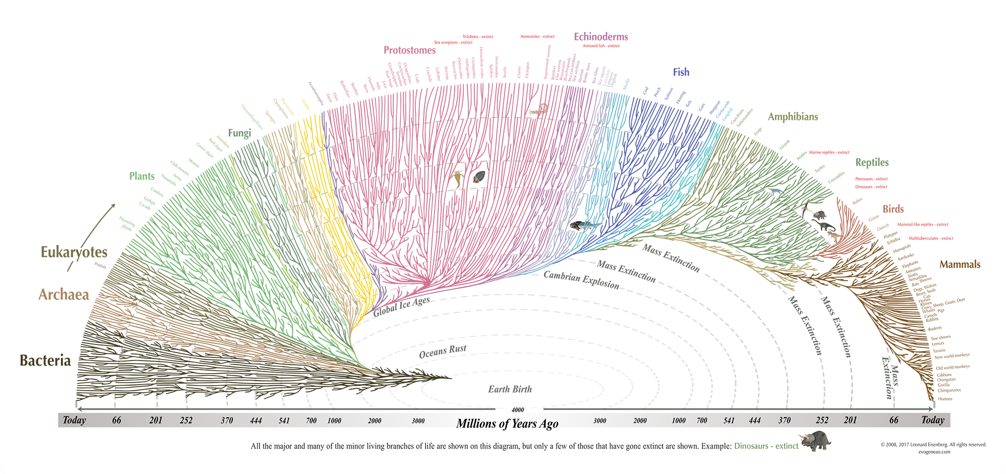
Eisenberg, L. (2018). The tree of life. Retrieved from: https://www.evogeneao.com/en
Masur, P. K. & Ranzini, G. (2023). Privacy Calculus, Privacy Paradox, and Context Collapse: A Replication of Three Key Studies in Communication Privacy Research. Manuscript in preparation.
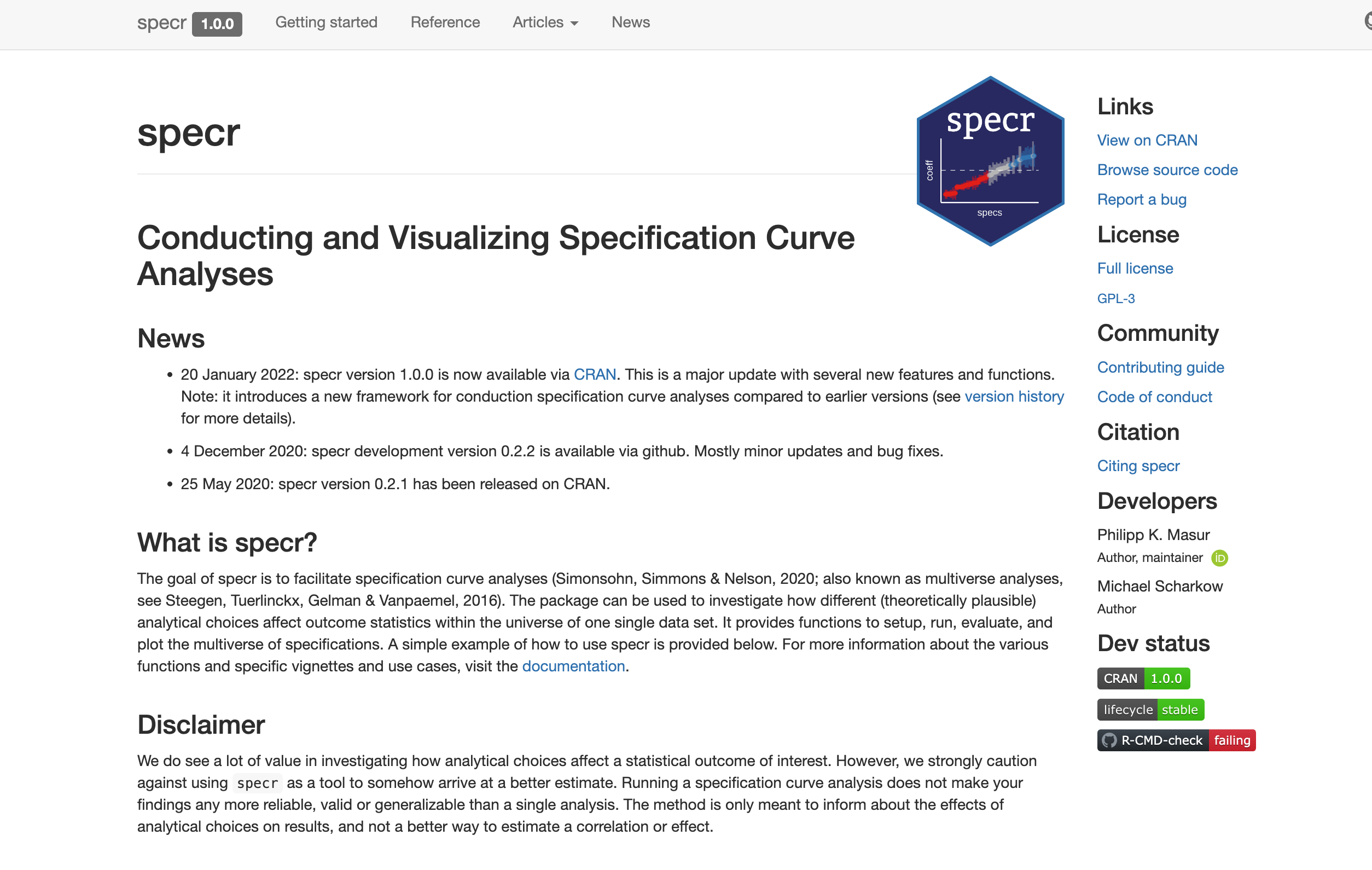
Masur, P. K. & Scharkow, M. (2020). specr: Conducting and Visualizing Specification Curve Analyses (R-package, version 1.0.0). https://CRAN.R-project.org/package=specr
McElreath, R. (2023). Statistical Rethinking 2023 - Horoscopes. Lecture on Youtube: https://www.youtube.com/watch?v=qwF-st2NGTU&t=224s
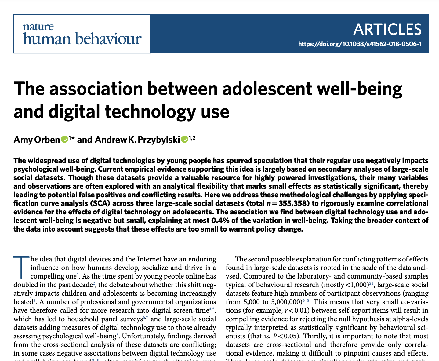
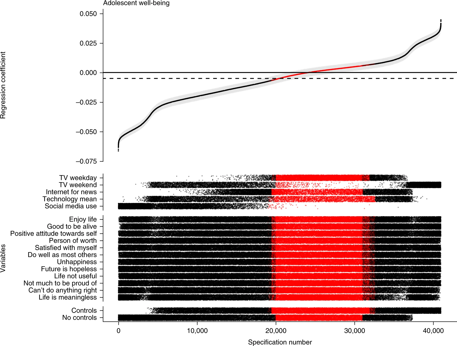
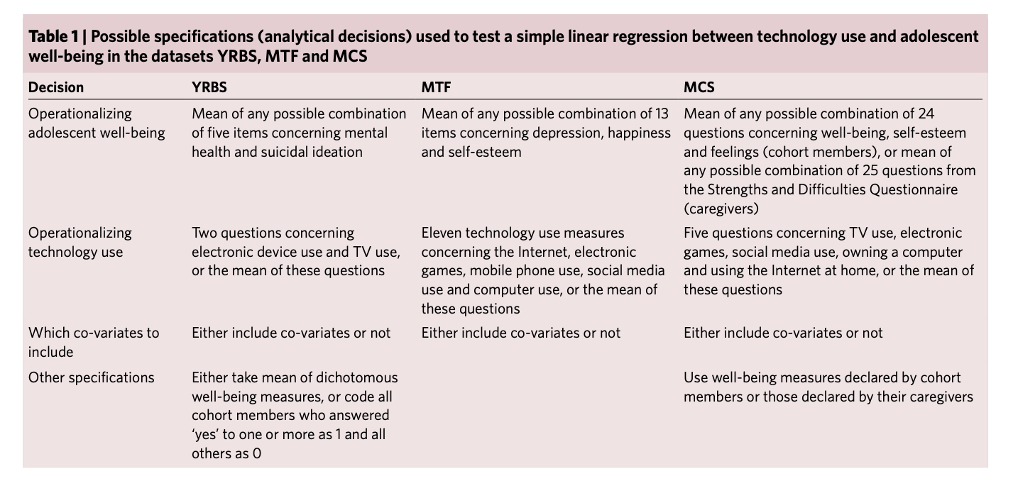
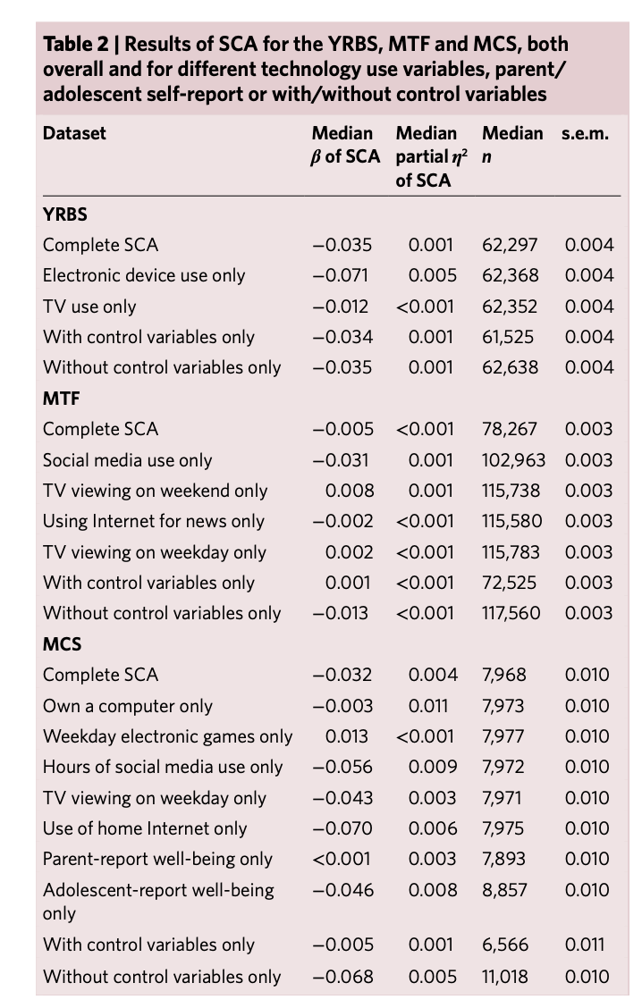
Orben, A., & Przybylski, A. K. (2019). The association between adolescent well-being and digital technology use. Nature human behaviour, 3(2), 173-182.
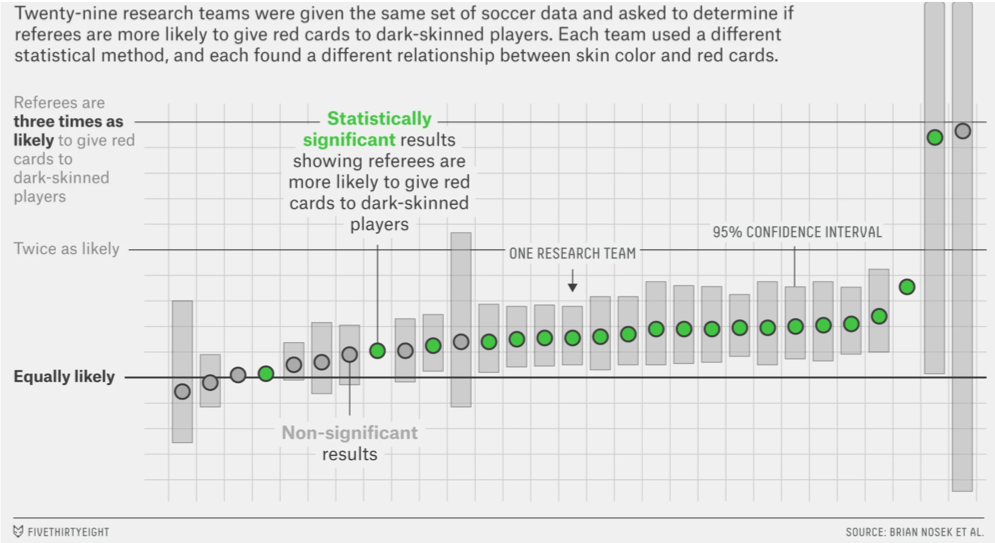
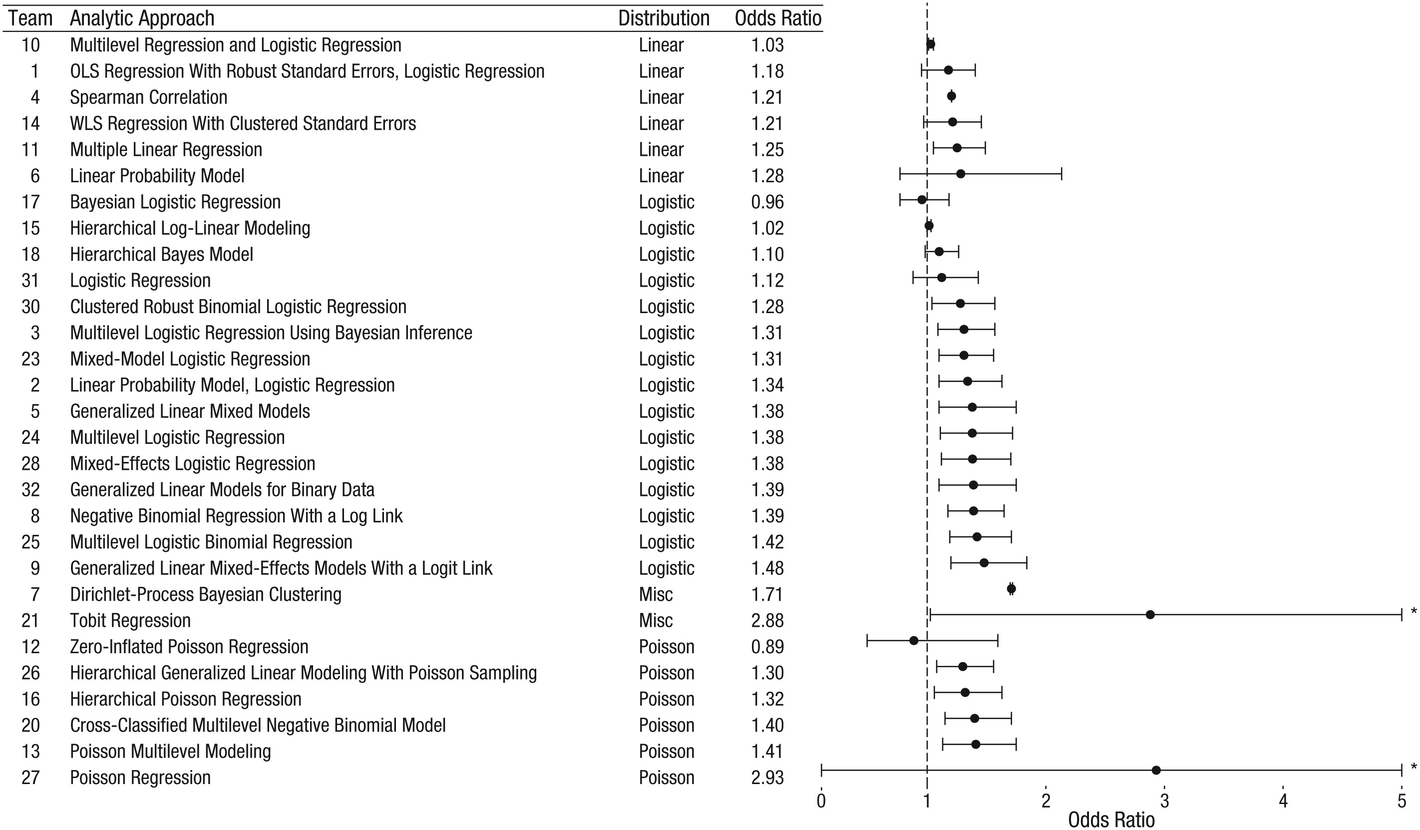
Silberzahn, R., Uhlmann, E. L., Martin, D. P., Anselmi, P., Aust, F., Awtrey, E., … & Nosek, B. A. (2018). Many analysts, one data set: Making transparent how variations in analytic choices affect results. Advances in Methods and Practices in Psychological Science, 1(3), 337-356.
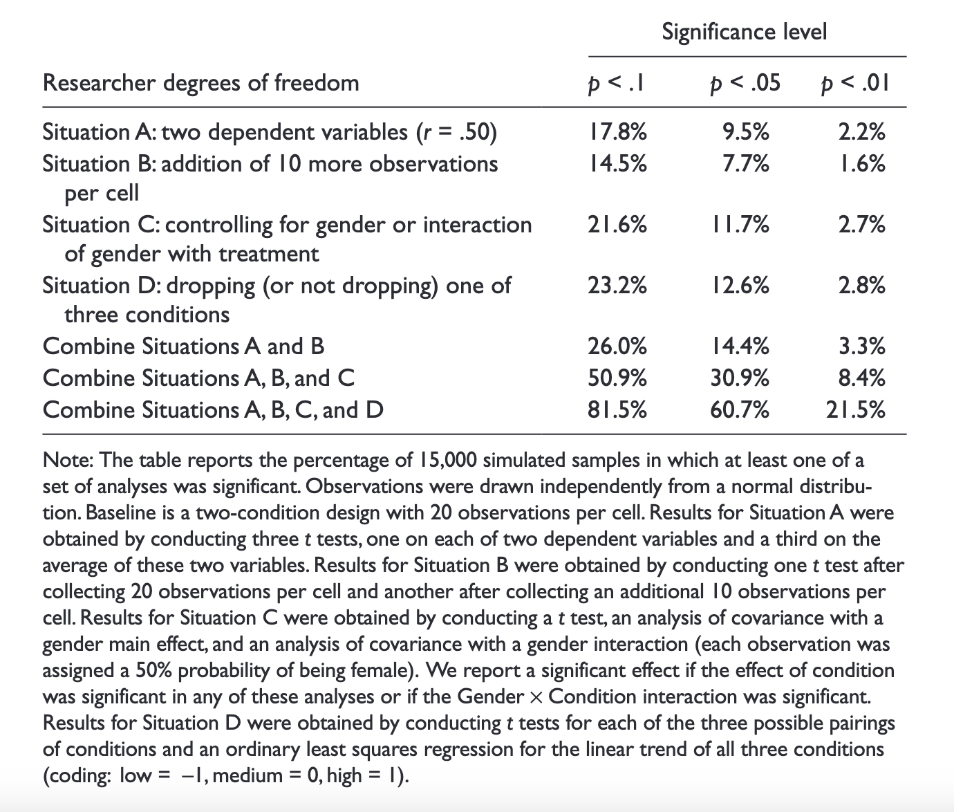
Simmons, J. P., Nelson, L. D., & Simonsohn, U. (2011). False-positive psychology: Undisclosed flexibility in data collection and analysis allows presenting anything as significant. Psychological science, 22(11), 1359-1366.
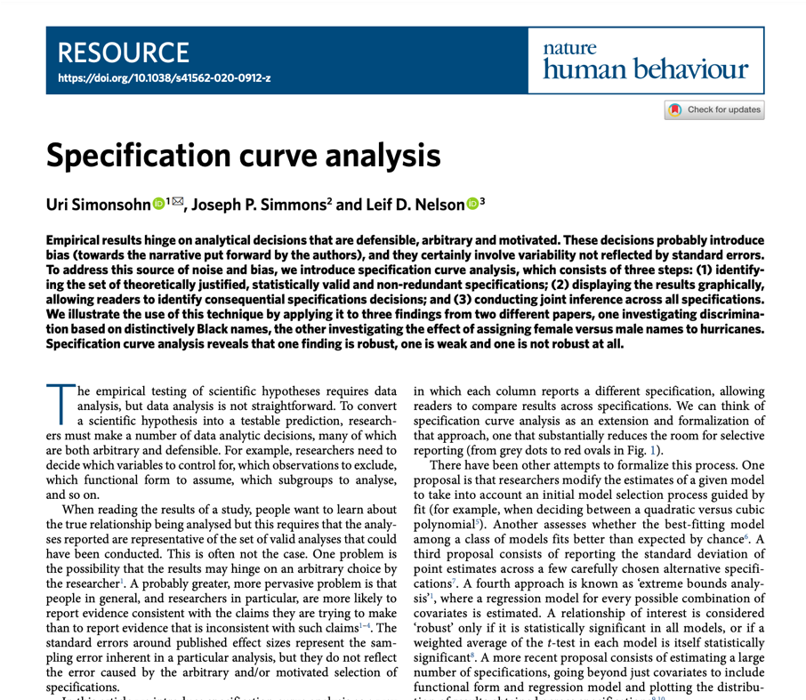
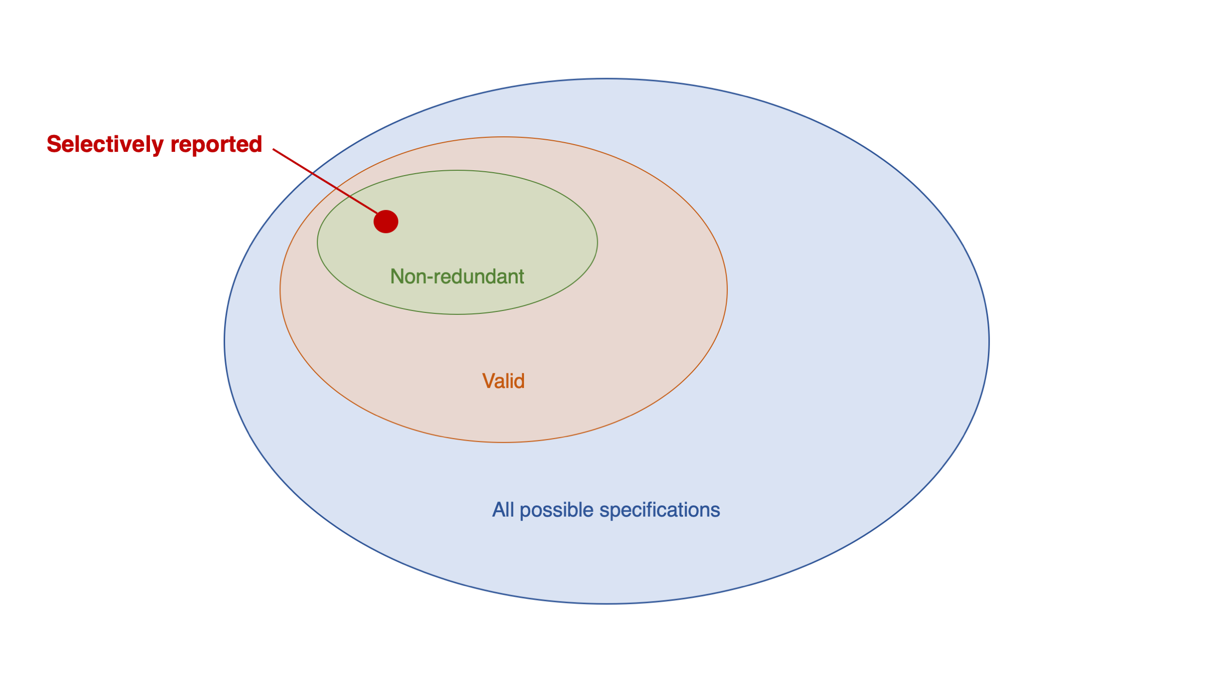
Simonsohn, U., Simmons, J.P. & Nelson, L.D. (2020). Specification curve analysis. Nature Human Behaviour, 4, 1208–1214. https://doi.org/10.1038/s41562-020-0912-z
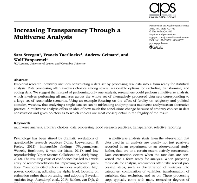
Steegen, S., Tuerlinckx, F., Gelman, A., & Vanpaemel, W. (2016). Increasing Transparency Through a Multiverse Analysis. Perspectives on Psychological Science, 11(5), 702-712. https://doi.org/10.1177/1745691616658637
.jpg/1024px-Sidney_Hall_-_Urania's_Mirror_-_Orion_(best_currently_available_version_-_2014).jpg)


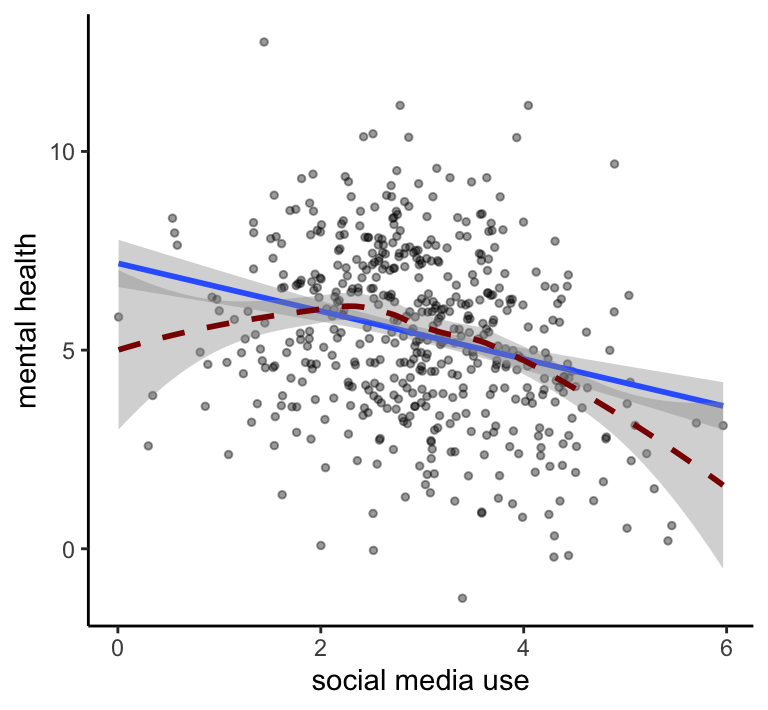


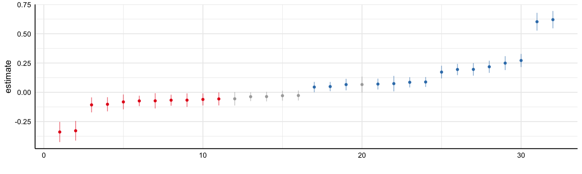


Social Media and Mental Health
Sampling 500 participants from a commercial online panel
Measuring social media use and mental health with (questionable) self-report measures
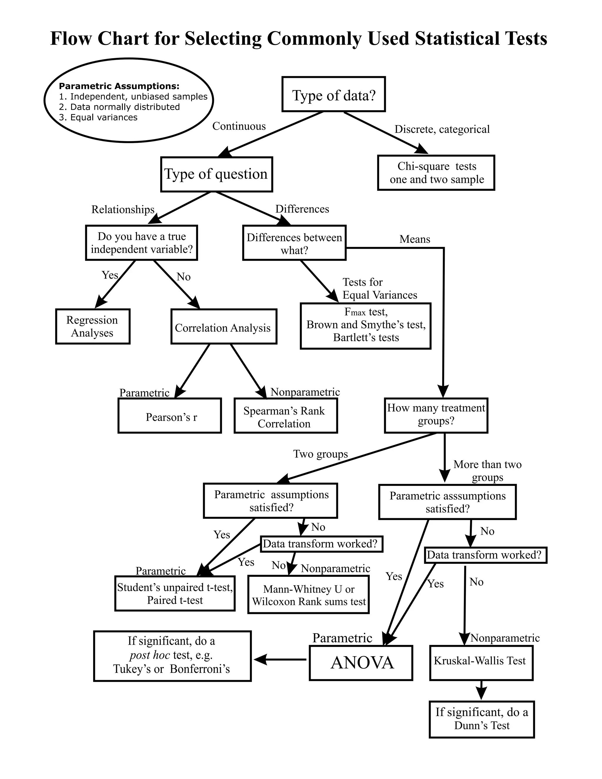
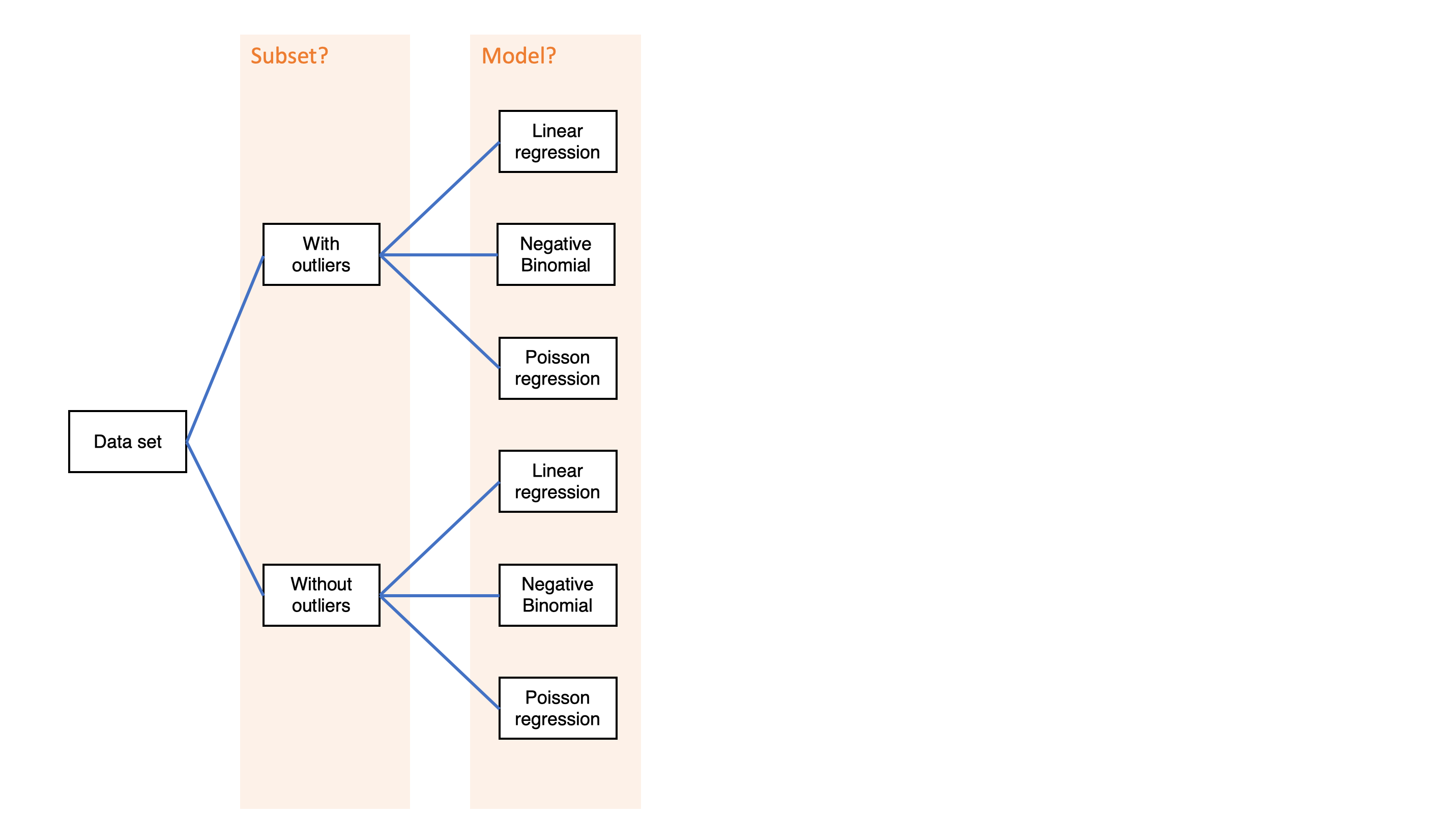
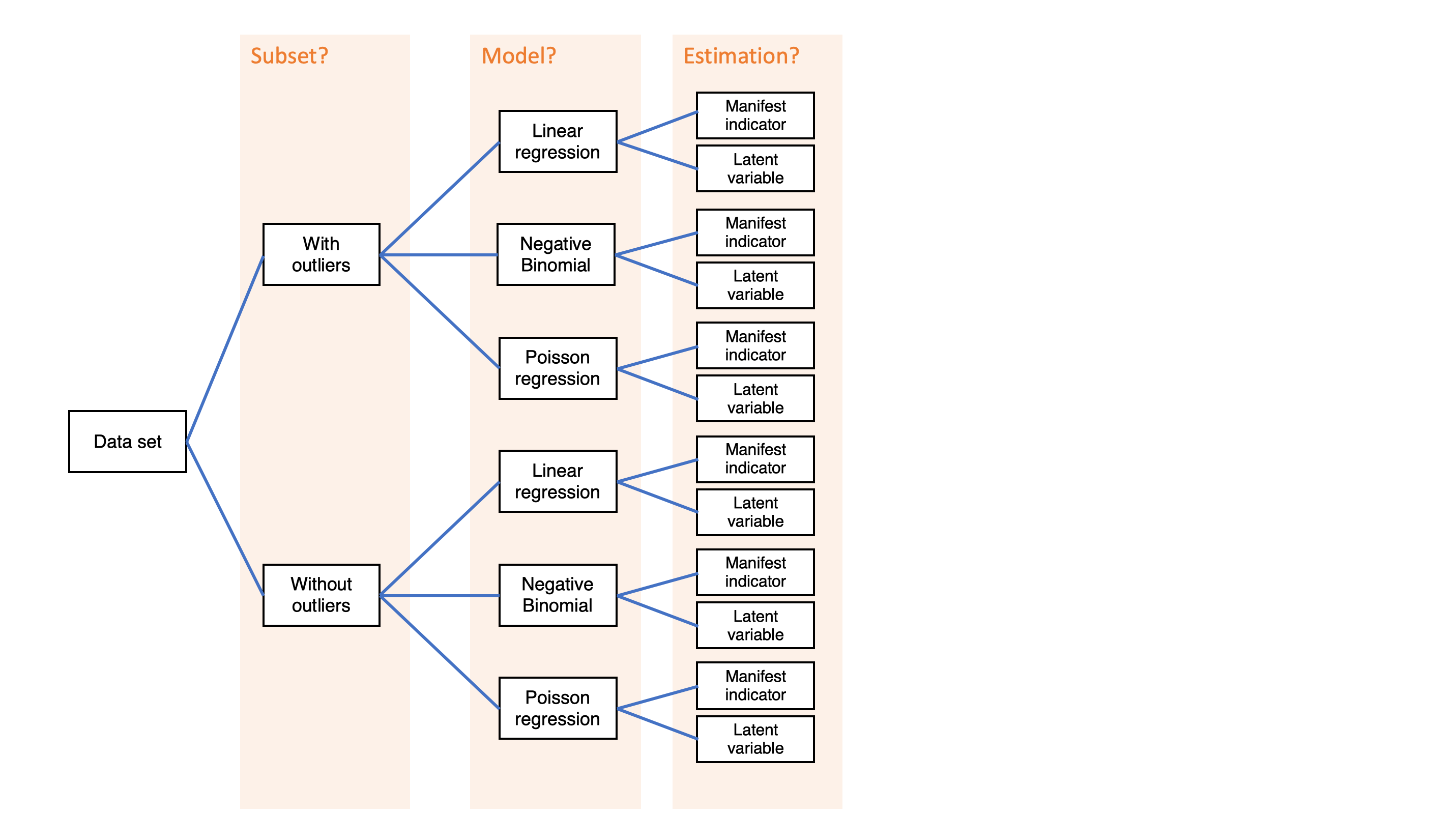
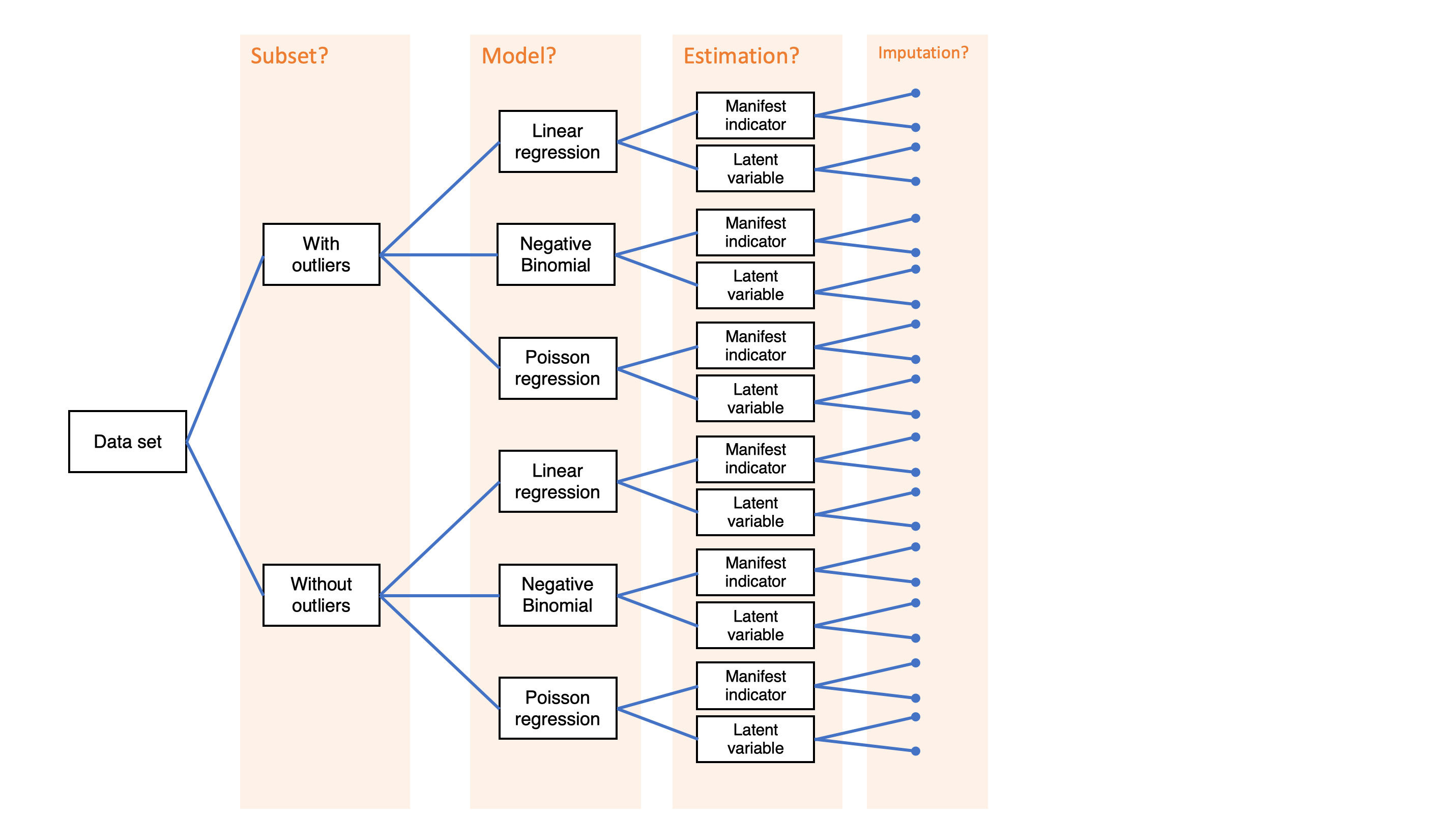
Simple decision path:
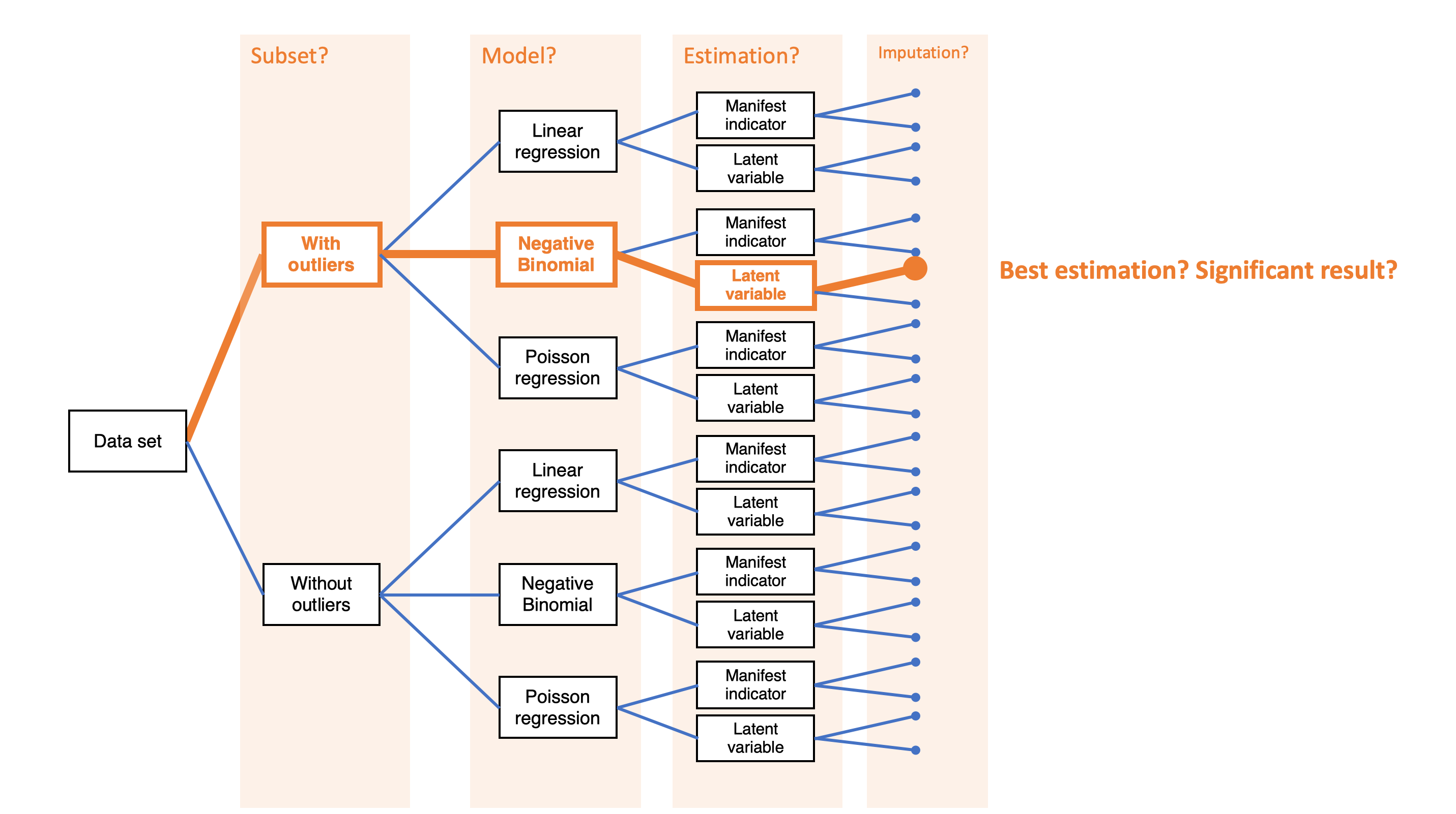
My choice: A (somewhat arbitrary) statistical model such as linear regression
My conclusion: Social media use is negatively related to mental health