In their paper, Simonsohn et al. (2020) propose a third step within the logic of specification curve analysis, which refers to conducting inference tests across the entire range of the specification curve. This step aims to address the following question: Considering the full set of reasonable specifications jointly, how inconsistent are the results with the null hypothesis of no effect?
We have been contemplating the implementation of this third step in our package. Until recently, we have concluded that there remains significant uncertainty regarding when such joint inferences are appropriate (see, for example, the recent discussion by Del Giudice & Gangestad, 2021), who highlight:
“In principle, multiverse-style analyses can be highly instructive. At the same time, analyses that explore multiverse spaces that are not homogeneous can produce misleading results and interpretations, lead scholars to dismiss the robustness of theoretically important findings that do exist, and discourage them from following fruitful avenues of research. This can hinder scientific progress just as much as the proliferation of false, unreplicable findings does” (p. 2).
The issue is as follows: Multiverse or specification curve analyses can serve different purposes. In the simplest form, it may serve to explore and discover differences in effect sizes that relate to specific theoretical or analytical decisions. Yet, the method is also suggestive of being a “somehow better approach to testing a relationship”. The aim of this second purpose, which is akin to a robustness test, is to exhaust the multiverse of truly arbitrary decisions in order to gain some sort of aggregate finding that can be use to refute or support a hypothesis. As Del Giudice and Gangestad point out very convincingly, however, it is often not straight-forward to decide whether specification is truly arbitrary (or in their terms: exhibits principled equivalence) compared to another specification. Yet, if this is not the case, running any inference tests is futile as “Just a few decisions incorrectly treated as arbitrary can quickly explode the size of the multiverse, drowning reasonable effect estimates in a sea of unjustified alternatives.” (Del Giudice & Gangestad, 2021, p. 2).
For these reasons, we have been, and continue to be, concerned that
tools for such an inference test could be misused or lead to improperly
conducted robustness tests. Nevertheless, due to frequent inquiries, we
have now integrated a function called boot_null() in the
latest development version of specr. For details on the
procedure, please refer to the paper by Simonsohn et al. (2020). Please
note that the implemented procedure pertains to the section “Inference
with non-experimental data” in the paper.
Preparations
Loading packages and data
For this tutorial, we will simple use the data set included in the
package, which we can call using example_data.
glimpse(example_data)
#> Rows: 1,000
#> Columns: 15
#> $ group1 <chr> "middle", "middle", "old", "old", "old", "middle", "middle", "y…
#> $ group2 <chr> "female", "male", "female", "female", "male", "male", "male", "…
#> $ group3 <chr> "C", "B", "A", "B", "A", "A", "C", "B", "C", "A", "C", "B", "A"…
#> $ x1     <dbl> 1.16616502, 0.76481253, -2.32781072, -0.50729975, -0.99903467, …
#> $ x2     <dbl> -0.36337844, 0.03490195, -0.99786005, -0.97004472, 0.54629183, …
#> $ x3     <dbl> -0.99899919, 0.12896300, -1.11167238, -0.08670481, 0.90082978, …
#> $ x4     <dbl> -0.29290911, -0.15539508, -1.27298782, -0.97830572, 2.56842916,…
#> $ c1     <dbl> 0.73628873, -0.72031278, 0.10362937, 1.78665608, -0.24463403, 0…
#> $ c2     <dbl> 0.17137360, 0.01651493, -2.89579197, -0.13769598, 2.02092928, -…
#> $ c3     <dbl> 0.2438919, -0.7708723, -6.9505025, -0.4307226, 2.8327862, -1.32…
#> $ c4     <dbl> 1.17397012, 0.00271097, 0.11513596, 0.84856292, -1.40719578, 0.…
#> $ y1     <dbl> -0.83896230, -1.19442262, -1.63184657, 0.20794834, -1.06889092,…
#> $ y2     <dbl> -1.15339449, -1.40708441, 0.46620798, 0.17421825, 2.89071414, 2…
#> $ y3     <dbl> -0.20911315, 0.17605870, -1.07664735, -0.37805585, -0.35389962,…
#> $ y4     <dbl> -0.10135448, -0.08908509, -0.27064865, 0.73415456, -0.20267287,…
Creating a custom function to extract full model
To prepare the inference under-the-null bootstrapping procedure, we
need to run the standard specification curve analysis, but make sure
that we keep the entire model object. By default, the function
specr() only keeps the relevant coefficient, but by
creating a customized fitting function, we can add a column that
contains the full model.
Setup specifications
When setting up the specifications, we simply pass the customized
function via the argument fun1.
Run standard specification curve analysis
Next, we simply ran the standard specification curve analysis using
the core function specr.
results <- specr(specs)
summary(results)
#> Results of the specification curve analysis
#> -------------------
#> Technical details:
#>
#>   Class:                          specr.object -- version: 1.0.1
#>   Cores used:                     1
#>   Duration of fitting process:    0.265 sec elapsed
#>   Number of specifications:       16
#>
#> Descriptive summary of the specification curve:
#>
#>  median  mad   min  max   q25  q75
#>    0.14 0.44 -0.34 0.62 -0.13 0.35
#>
#> Descriptive summary of sample sizes:
#>
#>  median  min  max
#>    1000 1000 1000
#>
#> Head of the specification results (first 6 rows):
#>
#> # A tibble: 6 × 25
#>   x     y     model controls      subsets formula   estimate std.error statistic
#>   <chr> <chr> <chr> <chr>         <chr>   <glue>       <dbl>     <dbl>     <dbl>
#> 1 x1    y1    lm    no covariates all     y1 ~ x1 …     0.62      0.04     16.4
#> 2 x1    y1    lm    c1            all     y1 ~ x1 …     0.6       0.04     15.6
#> 3 x1    y1    lm    c2            all     y1 ~ x1 …     0.61      0.04     15.9
#> 4 x1    y1    lm    c1 + c2       all     y1 ~ x1 …     0.59      0.04     15.1
#> 5 x1    y2    lm    no covariates all     y2 ~ x1 …    -0.33      0.04     -7.68
#> 6 x1    y2    lm    c1            all     y2 ~ x1 …    -0.34      0.04     -7.72
#> # ℹ 16 more variables: p.value <dbl>, conf.low <dbl>, conf.high <dbl>,
#> #   res <list>, fit_r.squared <dbl>, fit_adj.r.squared <dbl>, fit_sigma <dbl>,
#> #   fit_statistic <dbl>, fit_p.value <dbl>, fit_df <dbl>, fit_logLik <dbl>,
#> #   fit_AIC <dbl>, fit_BIC <dbl>, fit_deviance <dbl>, fit_df.residual <dbl>,
#> #   fit_nobs <dbl>
So far, nothing new. We get the results of the specification curve analysis and can explore them descriptively or visually.
Refit the models under-the-null
The idea behind this inference approach is that one forces the null on the data. Have a look at the following section of the Simonsohn et al. (2020) paper (p. 1213):
Run bootstrap sampling procedure
To run this procedure, we simply use the function
boot_null(), which requires the results, the specification
setup, and the number of samples that should be drawn (Simonsohn et
al. suggest n_samples = 500, here I am only demonstrating it with 10
resamples). Technically, we would suggest to run at least 1,000 or
better 10,000 samples to obtain robust results (as is common in
bootstrapping procedures or Monte Carlo simulations).
set.seed(42)
boot_models <- boot_null(results, specs, n_samples = 10) # better 1,000 - 10,000!
boot_models
#> Results of bootstrapping 'under-the-null' procedure
#> -------------------
#> Technical details:
#>
#>   Class:                           specr.boot -- version: 1.0.1
#>   Cores used:                      1
#>   Duration of fitting process:     20.001 sec elapsed
#>   Number of bootstrapped samples:  10
#>
#> Descriptive summary of the specification curves 'under-the-null' (head):
#>
#>           id median   min  max
#>  Bootstrap01  -0.01 -0.14 0.06
#>  Bootstrap02   0.00 -0.08 0.02
#>  Bootstrap03  -0.02 -0.12 0.02
#>  Bootstrap04  -0.03 -0.10 0.02
#>  Bootstrap05   0.00 -0.05 0.09
#>  Bootstrap06   0.00 -0.08 0.06
#>
#>
#> Overall median across all resamples (should be close to NULL):
#>
#>  median   min   max
#>   -0.01 -0.01 -0.01
The resulting fit object includes all resamples under the null (the output shows the first 6 curves summarized).
Summarize findings
Based on these resamples, we can compute several test statistics. Simonsohn et al. propose three, but we implemented the first two for now:
Obtaining the median effect estimated across all specifications, and then testing whether this median estimated effect is more extreme than would be expected if all specifications had a true effect of zero.
The share of specifications that obtain a statistically significant effect in the predicted direction, testing whether such share is more extreme (higher) than would be expected if all specifications had an effect of zero.
These test statistics can be obtained by simply using the generic
function summary() around the fitted bootstrap object:
summary(boot_models)
#> # A tibble: 3 × 3
#>   type           estimate p.value
#>   <chr>          <chr>    <chr>
#> 1 median         0.14     < .001
#> 2 share positive 8 / 16   < .001
#> 3 share negative 6 / 16   < .001
As we can see here, first, the likelihood of obtaining a median of 0.14 under the assumption that all specifications had a true effect of zero is very low (p < .001). Furthermore, 8 out of 16 specifications are actually in the right direction and the likelihood of this share of specifications that obtains a statistically significant effect in the predicted direction (here: positive) to be obtained if the true effect was zero is again low (p < .001).
Plot inference curve
Simonsohn et al. also suggest that the observed specification curve can be plotted against the expected under-the-null specification curves. In the figure, we see three expected curves that are based on the 10 resamples under-the-null (if more resamples are drawn, they are based on those resamples). The three curves here represent the 2.5th (low), the 50th (mid) and the 97.5th percentiles of these resamples.
plot(boot_models)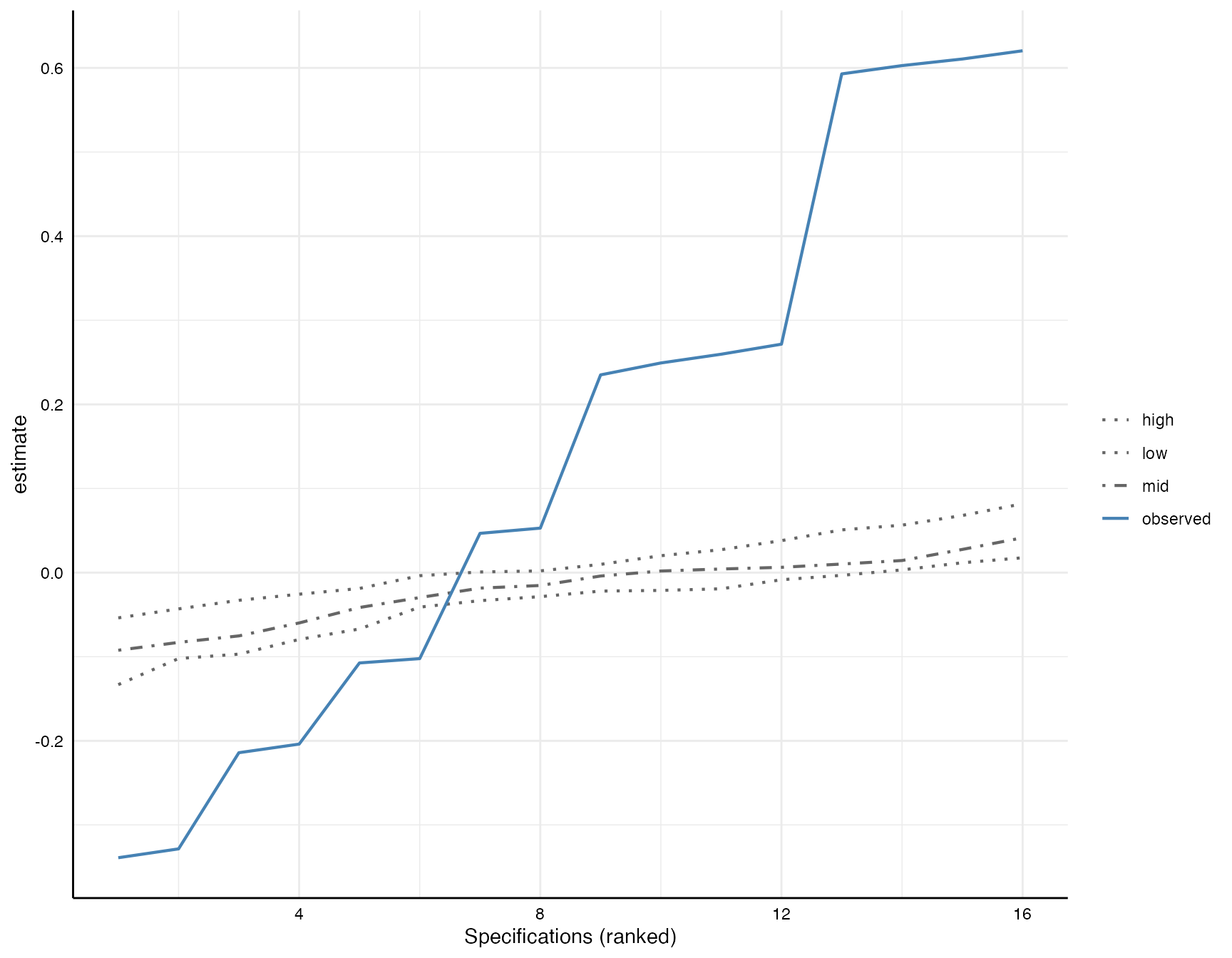
As we can see, the observed curve is clearly different than the simulated curves unter the assumption that the true effect is zero.
References
Del Giudice, M., & Gangestad, S. W. (2021). A traveler’s guide to the multiverse: Promises, pitfalls, and a framework for the evaluation of analytic decisions. Advances in Methods and Practices in Psychological Science, 4(1), https://journals.sagepub.com/doi/full/10.1177/2515245920954925.
Simonsohn, U., Simmons, J.P. & Nelson, L.D. (2020). Specification curve analysis. Nature Human Behaviour, 4, 1208–1214. https://doi.org/10.1038/s41562-020-0912-z