Investigating specific specifications • specr

Per default, specr() summarizes individual specifications by using broom::tidy() and broom::glance(). For most cases, this provides a sufficient and appropriate summary of the relationship of interest and model characteristics. Sometimes, however, it might be useful to investigate specific models in more detail or to investigate a specific parameter that is not provided by the two functions (e.g., r-square). This vignette shows how to access individual models and extract further information from them.

library(tidyverse)
library(specr)
library(performance)

Setup specifications with a specific extract function

If we want to investigate individual models and particularly all aspects of that model, we need to create a custom extract function that also stores the entire model object in the result data frame.

# Custom function
tidy_new <- function(x) {
  fit <- broom::tidy(x, conf.int = TRUE)
  fit$res <- list(x)  # Store model object
  return(fit)
}

# Run specification curve analysis
specs <- setup(data = example_data, 
               y = c("y1", "y2"), 
               x = c("x1", "x2"), 
               model = c("lm"),
               controls = c("c1", "c2"),
               subsets = list(group1 = unique(example_data$group1),  
                              group2 = unique(example_data$group2)),
               fun1 = tidy_new)

results <- specr(specs)

Identify model(s) of interest

For this example, we are going to look at two specific models (same independent variables, all controls, all participants, but different dependent variables).

(y_models <- results %>%
  as_tibble %>%
  filter(x == "x1", 
         controls == "c1 + c2",
         subsets == "all")) %>%
  select(x:group2, estimate:res)
#> # A tibble: 2 × 14
#>   x     y     model controls subsets group1 group2 estimate std.error statistic
#>   <chr> <chr> <chr> <chr>    <chr>   <fct>  <fct>     <dbl>     <dbl>     <dbl>
#> 1 x1    y1    lm    c1 + c2  all     NA     NA        0.593    0.0393     15.1 
#> 2 x1    y2    lm    c1 + c2  all     NA     NA       -0.214    0.0389     -5.51
#> # ℹ 4 more variables: p.value <dbl>, conf.low <dbl>, conf.high <dbl>,
#> #   res <list>

As you can see, the resulting tibble includes an additional column called res. This column includes the entire “model object” and we can use it to further investigate each model.

Investigate models

For example, we can now easily get a full summary of the models and compare individual coefficients and statistics.

y_models %>%
  pull(res) %>%
  map(summary) %>%
  map(coef)
#> [[1]]
#>                Estimate Std. Error    t value      Pr(>|t|)
#> (Intercept) -1.09466509 0.03582021 -30.559989 3.127670e-145
#> x1           0.59291826 0.03933279  15.074403  2.084917e-46
#> c1           0.06781034 0.03327698   2.037756  4.183823e-02
#> c2          -0.04278267 0.03079000  -1.389499  1.649916e-01
#> 
#> [[2]]
#>                Estimate Std. Error   t value     Pr(>|t|)
#> (Intercept)  0.79394670 0.03540987 22.421621 1.828378e-90
#> x1          -0.21413105 0.03888221 -5.507172 4.640637e-08
#> c1           0.03921893 0.03289578  1.192218 2.334599e-01
#> c2           0.54186302 0.03043728 17.802607 9.085852e-62

Or we could get r-squared values for both models (here using the function r2() from the performance package).

y_models %>%
  pull(res) %>% 
  map(r2)       # r2 is include in the package "performance"
#> [[1]]
#> # R2 for Linear Regression
#>        R2: 0.217
#>   adj. R2: 0.215
#> 
#> [[2]]
#> # R2 for Linear Regression
#>        R2: 0.285
#>   adj. R2: 0.282

Some more examples

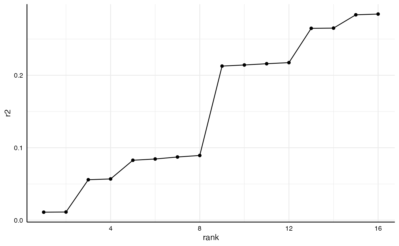
This way, we can analyze or compare such statistics across several models.

r2_results <- results %>%
  as_tibble %>%
  filter(subsets == "all") %>%
  mutate(r2 = map(res, r2), 
         r2 = map_dbl(r2, 1)) %>%
  arrange(r2)

r2_results %>%
  select(x:controls, r2)
#> # A tibble: 16 × 5
#>    x     y     model controls          r2
#>    <chr> <chr> <chr> <chr>          <dbl>
#>  1 x2    y2    lm    no covariates 0.0110
#>  2 x2    y2    lm    c1            0.0112
#>  3 x1    y2    lm    no covariates 0.0558
#>  4 x1    y2    lm    c1            0.0569
#>  5 x2    y1    lm    no covariates 0.0827
#>  6 x2    y1    lm    c2            0.0844
#>  7 x2    y1    lm    c1            0.0872
#>  8 x2    y1    lm    c1 + c2       0.0893
#>  9 x1    y1    lm    no covariates 0.213 
#> 10 x1    y1    lm    c2            0.214 
#> 11 x1    y1    lm    c1            0.216 
#> 12 x1    y1    lm    c1 + c2       0.217 
#> 13 x2    y2    lm    c2            0.265 
#> 14 x2    y2    lm    c1 + c2       0.265 
#> 15 x1    y2    lm    c2            0.284 
#> 16 x1    y2    lm    c1 + c2       0.285

And we can plot comparisons…

r2_results %>%
  arrange(r2) %>%
  mutate(rank = 1:n()) %>%
  ggplot(aes(x = rank, 
             y = r2)) +
  geom_point() +
  geom_line() +
  theme_minimal() +
  theme(strip.text = element_blank(),
        axis.line = element_line("black", size = .5),
        axis.text = element_text(colour = "black"))
#> Warning: The `size` argument of `element_line()` is deprecated as of ggplot2 3.4.0.
#> ℹ Please use the `linewidth` argument instead.
#> This warning is displayed once every 8 hours.
#> Call `lifecycle::last_lifecycle_warnings()` to see where this warning was
#> generated.