Many data are hierarchical and we want to acknowledge the nested
structure in our models. Specr can easily estimate such multilevel
models. We again have to write a customized function that we can pass
first to setup() and the specr() will do the
rest.
For this example, we will us the gapminder data set that
is included in the gapminder
package. We quickly recode some variable to get more interpretable
estimates.
# Load packages
library(tidyverse)
library(specr)
library(gapminder)
library(lme4)

# Recode some variables
gapminder <- gapminder %>%
  mutate(gdpPercap_log = log(gdpPercap),
         pop = pop/1000)

# Check data
head(gapminder)
#> # A tibble: 6 × 7
#>   country     continent  year lifeExp    pop gdpPercap gdpPercap_log
#>   <fct>       <fct>     <int>   <dbl>  <dbl>     <dbl>         <dbl>
#> 1 Afghanistan Asia       1952    28.8  8425.      779.          6.66
#> 2 Afghanistan Asia       1957    30.3  9241.      821.          6.71
#> 3 Afghanistan Asia       1962    32.0 10267.      853.          6.75
#> 4 Afghanistan Asia       1967    34.0 11538.      836.          6.73
#> 5 Afghanistan Asia       1972    36.1 13079.      740.          6.61
#> 6 Afghanistan Asia       1977    38.4 14880.      786.          6.67
Simply adding a random effect structure
For this example, we use the package lme4 and more
specifically the function lmer() to estimate the multilevel
model (more complex models such as poisson or negative binomial
multilevel models can likewise be estimated).
Based on the data set, we want to estimate the relationship between
gdpPercap (GDP per capita) and lifeExp (life
expectancy). Both variables are nested within both countries and years.
We can simply add a respective random effect structure via the argument
add_to_formula. This way, this will be automatically
included in the formula of all specifications. Because
broom doesn’t provide a tidy function for
merMod-objects resulting from lme4::lmer(), we
need to add a new extraction function like so
fun1 = new_function. Luckily, we can use the
broom.mixed package, which agian provides a tidy function
for such objects.
specs <- setup(data = gapminder,
                y = c("lifeExp"),
                x = c("gdpPercap_log"),
                model = c("lmer"),
                controls = "pop",
                fun1 = function(x) broom.mixed::tidy(x, conf.int = TRUE),
                add_to_formula = "(1|country) + (1|year)")

# Check formula
summary(specs)
#> Setup for the Specification Curve Analysis
#> -------------------------------------------
#> Class:                      specr.setup -- version: 1.0.1
#> Number of specifications:   2
#>
#> Specifications:
#>
#>   Independent variable:     gdpPercap_log
#>   Dependent variable:       lifeExp
#>   Models:                   lmer
#>   Covariates:               no covariates, pop
#>   Subsets analyses:         all
#>
#> Function used to extract parameters:
#>
#>   function(x) broom.mixed::tidy(x, conf.int = TRUE)
#>
#>
#> Head of specifications table (first 6 rows):
#> # A tibble: 2 × 6
#>   x             y       model controls      subsets formula
#>   <chr>         <chr>   <chr> <chr>         <chr>   <glue>
#> 1 gdpPercap_log lifeExp lmer  no covariates all     lifeExp ~ gdpPercap_log + 1…
#> 2 gdpPercap_log lifeExp lmer  pop           all     lifeExp ~ gdpPercap_log + p…

# Run analysis and inspect results
results <- specr(specs)
#> Warning: There was 1 warning in `dplyr::mutate()`.
#> ℹ In argument: `out = pmap(...)`.
#> Caused by warning:
#> ! Some predictor variables are on very different scales: consider rescaling
as_tibble(results)
#> # A tibble: 2 × 22
#>   x       y     model controls subsets formula model_function effect group term
#>   <chr>   <chr> <chr> <chr>    <chr>   <glue>  <list>         <chr>  <chr> <chr>
#> 1 gdpPer… life… lmer  no cova… all     lifeEx… <fn>           fixed  NA    gdpP…
#> 2 gdpPer… life… lmer  pop      all     lifeEx… <fn>           fixed  NA    gdpP…
#> # ℹ 12 more variables: estimate <dbl>, std.error <dbl>, statistic <dbl>,
#> #   conf.low <dbl>, conf.high <dbl>, fit_nobs <int>, fit_sigma <dbl>,
#> #   fit_logLik <dbl>, fit_AIC <dbl>, fit_BIC <dbl>, fit_REMLcrit <dbl>,
#> #   fit_df.residual <int>
Defining customatized multilevel functions
Sometimes, we may not want to add one random effect structure to all models and instead explore more specific random structure (and even several different random effect structures). In this case, we create several customized lmer-functions that account for different nesting structures.
# Random intercept model (only country as grouping variable)
lmer_ri_1 <- function(formula, data,...) {
require(lme4)
require(broom.mixed)
formula <- paste(formula, "+ (1|country)")
lmer(formula, data)
}
# Including random slopes (only country as grouping variable)
lmer_rs_1 <- function(formula, data,...) {
require(lme4)
require(broom.mixed)
slopevars <- unlist(strsplit(formula, " ~ "))[2]
formula <- paste0(formula, "+ (1 + ", slopevars, "|country)" )
lmer(formula, data)
}
# Random intercept model (lifeExp is nested in both countries and years)
lmer_ri_2 <- function(formula, data,...) {
require(lme4)
require(broom.mixed)
formula <- paste0(formula, "+ (1|country) + (1|year)")
lmer(formula, data)
}
# Including random slopes (intercept and slopes are nested in both countries and years)
lmer_rs_2 <- function(formula, data,...) {
require(lme4)
require(broom.mixed)
slopevars <- unlist(strsplit(formula, " ~ "))[2]
formula <- paste0(formula, "+ (1 + ", slopevars, "|country) + (", slopevars, "|year)" )
lmer(formula, data)
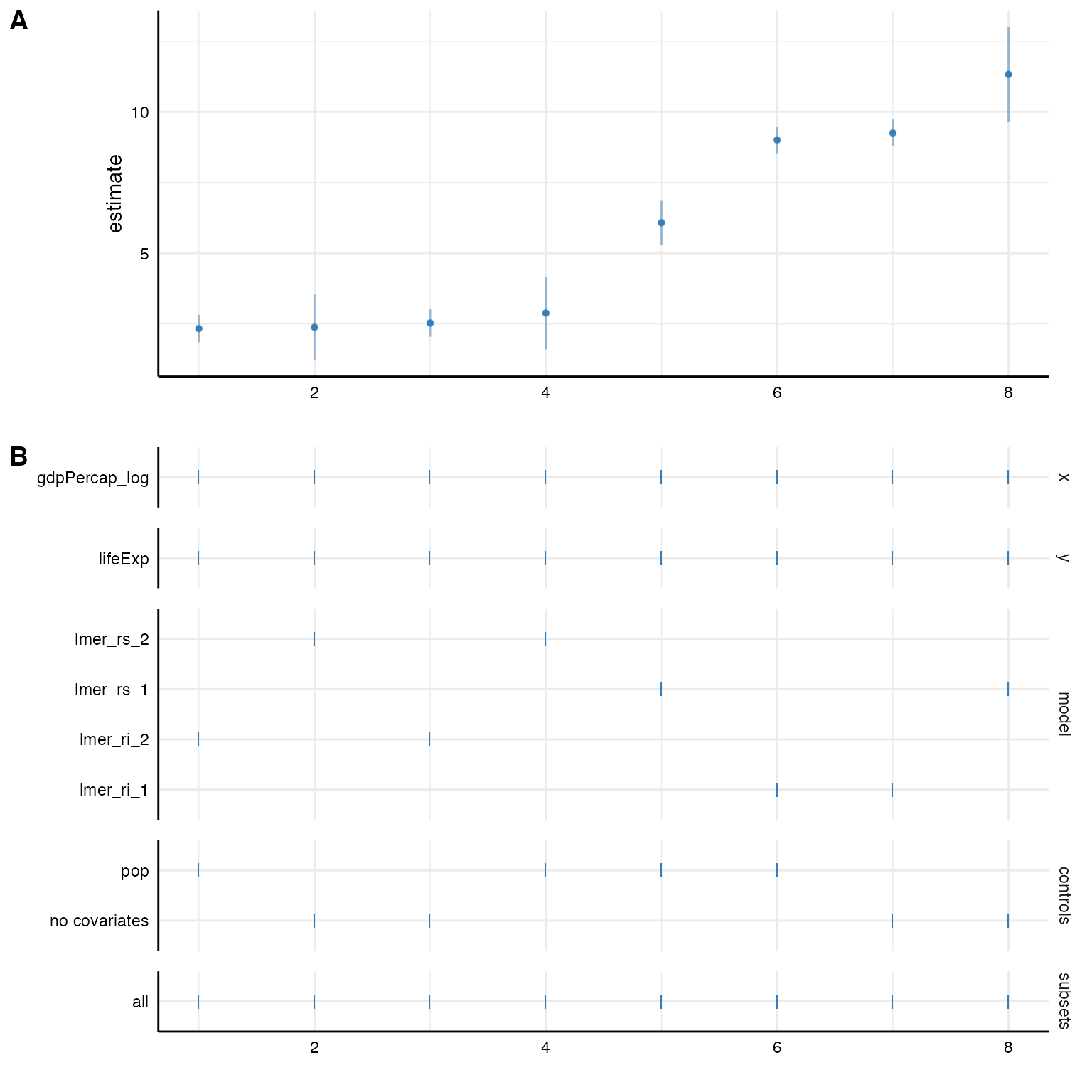
}Setting up specifications
We can now use these function to estimate these models. In this example, we investigate the influence of different nesting structures on the fixed effect between GDP per capita and life expectancy.
# Setup specifications with customized functions
specs <- setup(data = gapminder,
               y = c("lifeExp"),
               x = c("gdpPercap_log"),
               model = c("lmer_ri_1", "lmer_ri_2",
                         "lmer_rs_1", "lmer_rs_2"),
               controls = "pop")

# Check specifications
summary(specs)
#> Setup for the Specification Curve Analysis
#> -------------------------------------------
#> Class:                      specr.setup -- version: 1.0.1
#> Number of specifications:   8
#>
#> Specifications:
#>
#>   Independent variable:     gdpPercap_log
#>   Dependent variable:       lifeExp
#>   Models:                   lmer_ri_1, lmer_ri_2, lmer_rs_1, lmer_rs_2
#>   Covariates:               no covariates, pop
#>   Subsets analyses:         all
#>
#> Function used to extract parameters:
#>
#>   function (x)
#> broom::tidy(x, conf.int = TRUE)
#> <environment: 0x7fc7fc4bce40>
#>
#>
#> Head of specifications table (first 6 rows):
#> # A tibble: 6 × 6
#>   x             y       model     controls      subsets formula
#>   <chr>         <chr>   <chr>     <chr>         <chr>   <glue>
#> 1 gdpPercap_log lifeExp lmer_ri_1 no covariates all     lifeExp ~ gdpPercap_log…
#> 2 gdpPercap_log lifeExp lmer_ri_1 pop           all     lifeExp ~ gdpPercap_log…
#> 3 gdpPercap_log lifeExp lmer_ri_2 no covariates all     lifeExp ~ gdpPercap_log…
#> 4 gdpPercap_log lifeExp lmer_ri_2 pop           all     lifeExp ~ gdpPercap_log…
#> 5 gdpPercap_log lifeExp lmer_rs_1 no covariates all     lifeExp ~ gdpPercap_log…
#> 6 gdpPercap_log lifeExp lmer_rs_1 pop           all     lifeExp ~ gdpPercap_log…