Plot variance decomposition

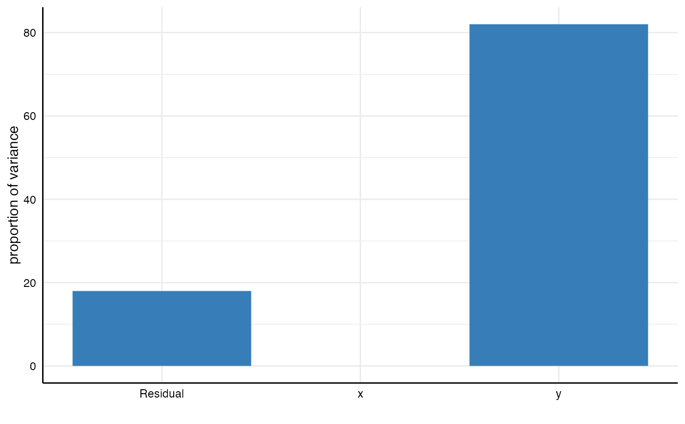
This function is deprecated because the new version of specr uses a new analytic framework. In this framework, you can plot a similar figure simply by using the generic plot() function and adding the argument type = "variance". This functions creates a simple barplot that visually displays how much variance in the outcome (e.g., the regression coefficient) different analytical choices or combinations therefor account for. To use this approach, one needs to estimate a multilevel model that includes all analytical choices as grouping variables (see examples and vignettes). This function uses icc_specs() to compute the intraclass correlation coefficients (ICCs), which provides the data basis for the plot (see examples).

plot_variance(model)

Arguments

model

a multilevel model that captures the variances of the specification curve (based on the data frame resulting from run_specs).

Value

a ggplot object.

See also

icc_specs() to produce a tibble that details the variance decomposition.

Examples

# Step 1: Run spec curve analysis
results <- run_specs(df = example_data,
                     y = c("y1", "y2"),
                     x = c("x1", "x2"),
                     model = c("lm"))

# Step 2: Estimate multilevel model
library(lme4, quietly = TRUE)
model <- lmer(estimate ~ 1 + (1|x)  + (1|y), data = results)

# Step 3: Plot model
plot_variance(model)
#> Warning: `plot_variance()` was deprecated in specr 1.0.0.
#> ℹ Please use `plot.specr.object()` instead.