Inference on the specification curve

Tests how inconsistent the specification curve as a whole is with the null hypothesis that the independent variable has no effect in any of the specifications. Following Simonsohn, Simmons and Nelson (2020, section "Inference with non-experimental data"), the function generates the distribution of specification curves that would be expected under the null by resampling data in which the null hypothesis is known to be true. 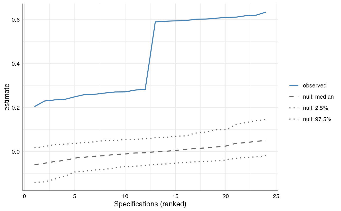The resulting object of class specr.infer can be summarized with summary() (test statistics and p-values) and plotted with plot() (observed curve against the curves under the null).

Usage

infer_curve(x, data, n_samples = 500, fast = TRUE, ...)

Arguments

x: A specr.object, resulting from running specr() (or the tibble that specr() returns when it is given a tibble of specifications).
data: The data set that was used to fit the specifications, or the specr.setup object created by setup() (whose data set is then used).
n_samples: Number of bootstrap samples drawn under the null. Defaults to 500. Use at least 1,000 for results that are reported.
fast: Logical value indicating whether specifications that were fitted with lm should be refitted with a fast least-squares routine. It gives the same estimates and p-values as lm(), which is checked against the observed results for every specification before it is used. Set to FALSE to refit all specifications with their original model function. Defaults to TRUE.
...: Further arguments passed to furrr::future_map(), e.g. .progress = TRUE. The argument .options cannot be set, because the resampling always uses furrr_options(seed = TRUE).

Value

An object of class specr.infer, a list that includes the observed curve (observed), the estimates and p-values under the null (estimates and p_values; matrices with one row per bootstrap sample and one column per specification), and technical information. Use methods(class = "specr.infer") for an overview on available methods.

Details

Procedure

For every specification k, the dependent variable is first modified so that the null hypothesis is true by construction: \(y^*_k = y_k - b_k x_k\), where \(b_k\) is the estimate observed in that specification. Then, in each of n_samples bootstrap samples, N rows are drawn with replacement from the data (N being the number of rows of data), and every specification is refitted on these rows with \(y^*_k\) as its dependent variable. The same rows are used for all specifications, which preserves the dependence between them. Each specification keeps its own model, control variables, subset, and additions to the formula, so that the curves under the null are based on exactly the same specifications as the observed curve.

Requirements

Because the null is imposed by subtracting \(b_k x_k\) from the dependent variable, the procedure is only valid for models that are linear in the dependent variable (e.g., lm, lmer, or glm with a gaussian family and identity link), for numeric independent and dependent variables, and for unstandardized estimates. Before resampling, infer_curve() refits every specification on the full data with \(y^*_k\) and stops if the estimate is not zero, which catches models and extraction functions for which this does not hold (e.g., logistic regression). Structural equation models (lavaan) are not supported. Note that rows are resampled independently, which ignores clustering (e.g., in multilevel data).

Interpretation

Joint inference across all specifications is only meaningful if the specifications are genuinely equivalent, arbitrary alternatives (Del Giudice & Gangestad, 2021). See vignette("inferences") for a discussion.

Parallelization

The bootstrap samples are distributed across workers if a parallel plan has been set up front, e.g. future::plan(future::multisession, workers = 4). Results are reproducible with set.seed() and identical whether they are computed sequentially or in parallel. For more information, see vignette("parallelization").

References

Simonsohn, U., Simmons, J.P. & Nelson, L.D. (2020). Specification curve analysis. Nature Human Behaviour, 4, 1208–1214. https://doi.org/10.1038/s41562-020-0912-z
Del Giudice, M., & Gangestad, S. W. (2021). A traveler’s guide to the multiverse: Promises, pitfalls, and a framework for the evaluation of analytic decisions. Advances in Methods and Practices in Psychological Science, 4(1). https://doi.org/10.1177/2515245920954925

Examples

# Setup and run specification curve analysis
specs <- setup(data = example_data,
   y = "y1",
   x = c("x1", "x2"),
   model = "lm",
   controls = c("c1", "c2"),
   subsets = list(group2 = c("female", "male")))

results <- specr(specs)

# Resample under the null (better 1,000 or more)
set.seed(42)
inference <- infer_curve(results, specs, n_samples = 200)

# Test statistics and p-values
summary(inference)
#> # A tibble: 3 × 6
#>   statistic                    estimate null_lower null_upper p.value n_specs
#>   <chr>                           <dbl>      <dbl>      <dbl>   <dbl>   <int>
#> 1 median                          0.437    -0.0578     0.0606 0.00498      24
#> 2 share significant (positive)   24         0          9      0.00498      24
#> 3 aggregated z                   45.6      -6.71       7.03   0.00498      24

# Observed curve against the curves under the null
plot(inference)


# For comparison: the same analysis after shuffling y1, which removes any
# effect of x1 and x2 in all specifications
shuffled <- example_data
shuffled$y1 <- sample(shuffled$y1)
specs_null <- setup(data = shuffled,
   y = "y1",
   x = c("x1", "x2"),
   model = "lm",
   controls = c("c1", "c2"),
   subsets = list(group2 = c("female", "male")))

summary(infer_curve(specr(specs_null), specs_null, n_samples = 200))
#> # A tibble: 3 × 6
#>   statistic                    estimate null_lower null_upper p.value n_specs
#>   <chr>                           <dbl>      <dbl>      <dbl>   <dbl>   <int>
#> 1 median                         0.0600    -0.0598     0.0757  0.0945      24
#> 2 share significant (positive)   5          0         10.0     0.134       24
#> 3 aggregated z                   6.22      -5.96       8.22    0.0945      24