Plot specification curve and analytical choices

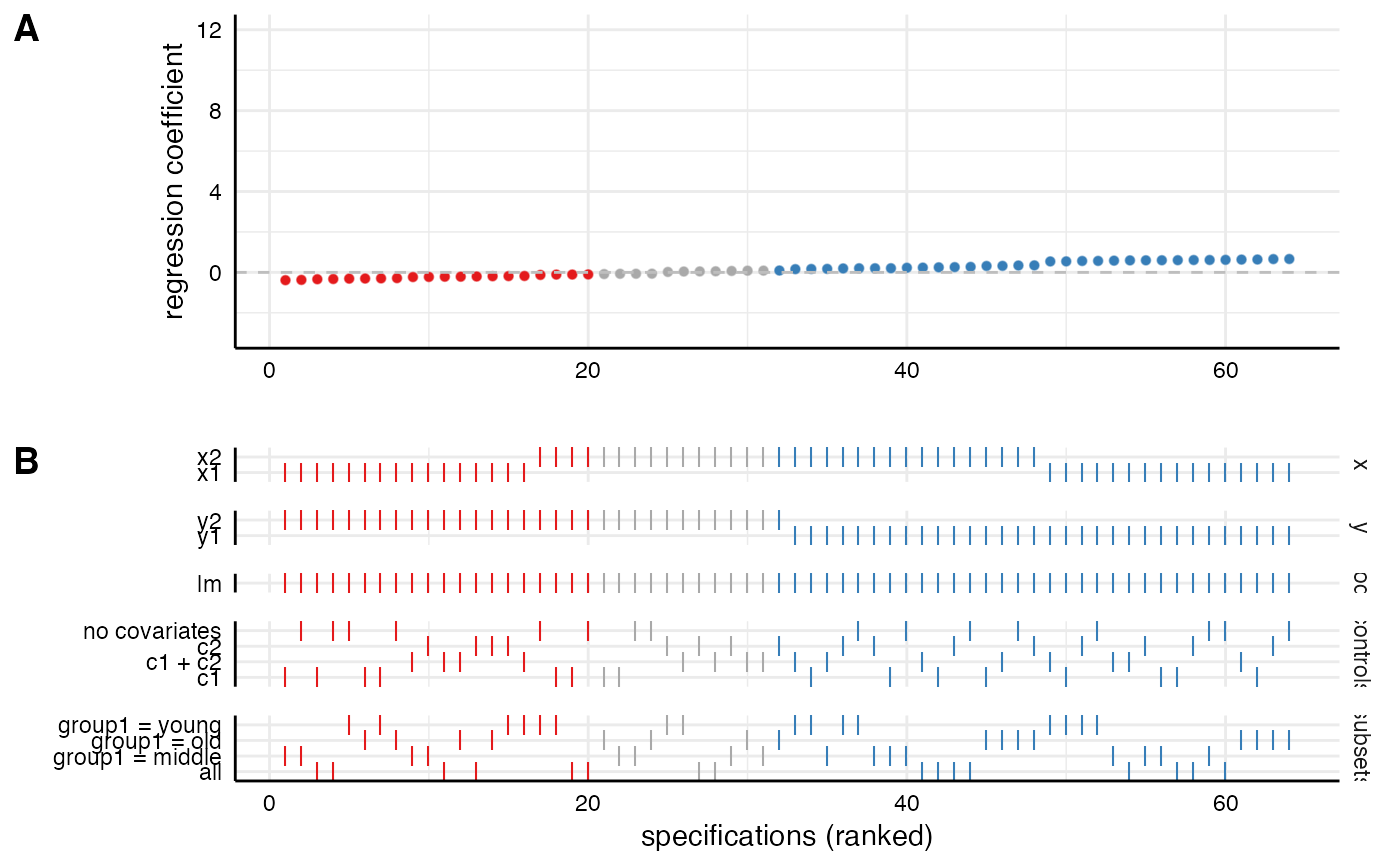
This function is deprecated because the new version of specr uses a new analytic framework. In this framework, you can plot a similar figure simply by using the generic plot() function and adding the argument type = "default".This function plots an entire visualization of the specification curve analysis. The function uses the entire tibble that is produced by run_specs() to create a standard visualization of the specification curve analysis. Alternatively, one can also pass two separately created ggplot objects to the function. In this case, it simply combines them using cowplot::plot_grid. 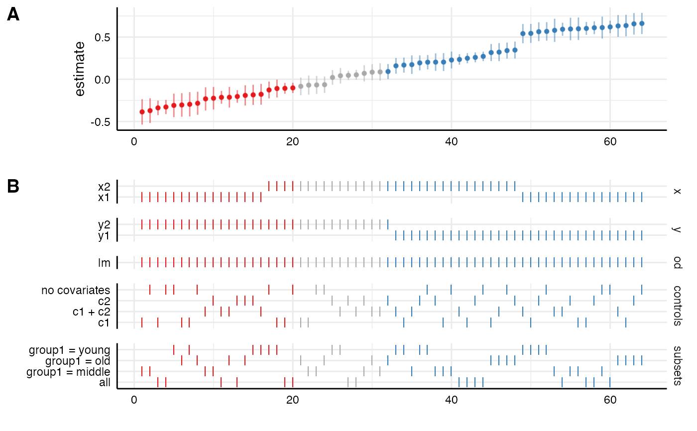Significant results are highlighted (negative = red, positive = blue, grey = nonsignificant).

plot_specs(
  df = NULL,
  plot_a = NULL,
  plot_b = NULL,
  choices = c("x", "y", "model", "controls", "subsets"),
  labels = c("A", "B"),
  rel_heights = c(2, 3),
  desc = FALSE,
  null = 0,
  ci = TRUE,
  ribbon = FALSE,
  ...
)

Arguments

df

a data frame resulting from run_specs().

plot_a

a ggplot object resulting from plot_curve() (or plot_choices() respectively).

plot_b

a ggplot object resulting from plot_choices() (or plot_curve() respectively).

choices

a vector specifying which analytical choices should be plotted. By default, all choices are plotted.

labels

labels for the two parts of the plot

rel_heights

vector indicating the relative heights of the plot.

desc

logical value indicating whether the curve should the arranged in a descending order. Defaults to FALSE.

null

Indicate what value represents the 'null' hypothesis (defaults to zero).

ci

logical value indicating whether confidence intervals should be plotted.

ribbon

logical value indicating whether a ribbon instead should be plotted.

...

additional arguments that can be passed to plot_grid().

Value

a ggplot object.

See also

• plot_curve() to plot only the specification curve.

• plot_choices() to plot only the choices panel.

• plot_samplesizes() to plot a histogram of sample sizes per specification.

Examples

# load additional library
library(ggplot2) # for further customization of the plots

# run spec analysis
results <- run_specs(example_data,
                     y = c("y1", "y2"),
                     x = c("x1", "x2"),
                     model = "lm",
                     controls = c("c1", "c2"),
                     subset = list(group1 = unique(example_data$group1)))

# plot results directly
plot_specs(results)
#> Warning: `plot_specs()` was deprecated in specr 1.0.0.
#> ℹ Please use `plot.specr.object()` instead.


# Customize each part and then combine
p1 <- plot_curve(results) +
  geom_hline(yintercept = 0, linetype = "dashed", color = "grey") +
  ylim(-3, 12) +
  labs(x = "", y = "regression coefficient")

p2 <- plot_choices(results) +
  labs(x = "specifications (ranked)")

plot_specs(plot_a = p1,    # arguments must be called directly!
           plot_b = p2,
           rel_height = c(2, 2))